2004-2005丹麦 质心法水下3D 距离选通成像

Underwater 3-D optical imaging with a gated viewing laser radar
Jens Busck
Danish Defence Research Establishment Ryvangs Alle 1
DK-2100Copenhagen Denmark and
Danish Technical University,?rsted DTU
?rsted Plads,Building 349DK-2800Kgs.Lyngby Denmark
E-mail:jb@ddre.dk
Abstract.New 3-D optical underwater images are presented.The 3-D images are recorded in fresh water and brackish sea water ?salinity 15‰?,at 4-to 5-m range.For the ?rst time,underwater 3-D images are computed by our new algorithm,which applies the method of weighted averages on a sequence of 2-D images.It is proposed that 3-D gated
viewing images can be recorded at any contrast
100%.A novel and dynamic way of measuring the is presented.A novel correction for gated viewing sented.For the ?rst time,an exact solution of the depth of gating is proposed for a rectangular laser pulse.?2005Society of Photo-Optical Instru-mentation Engineers.?DOI:10.1117/1.2127895?
Subject terms:underwater imaging;gated viewing;3-D images .
Paper 040960R received Dec.15,2004;revised manuscript received Apr.13,2005;accepted for publication Apr.18,2005;published online Nov.23,2005.
1Introduction
This work is a result of ongoing research at the Danish Defence Research Establishment and the Danish Technical University on the subject of optical identi?cation of sea mines.In general,sea mine recognition consists of an acoustic detection phase,an acoustic classi?cation phase,and an optical identi?cation phase.The performance of the optical imaging system is of crucial importance for correct
identi?cation.Faulty identi?cation may be lethal to the
divers going down with explosives to eliminate a sea mine.The Canadians 1built the laser underwater camera image enhancer ?LUCIE ?in 1993,and later an upgraded version ?LUCIE II ?with a faster camera.However,the LUCIE sys-tem captures only 2-D images by gated viewing.We prove in this work that this system could easily be processed into 3-D underwater images,since the Canadian and Danish systems are similar in several ways.The Swedes are well on the way to long-range gated viewing,up to an impres-sive 14-km range.2They do long-range 3-D imaging as well.3We proposed high accuracy,short-range gated view-ing 3-D imaging in 2004.4There exist several scanning and nonscanning techniques for optical laser imaging on land and underwater,among which just a few examples are the
streak tube imaging lidar,5–9staring focal plane array imag-ers ?e.g.,Ref.10?,pulsed infrared imagers ?e.g.,Ref.11?,amplitude modulated laser radar systems,12,13direct detec-tion laser vibrometry with an amplitude modulated ladar,14gated viewing with polarization,15etc.
The 3-D images and the algorithm presented in this work are a new step forward from the work of McLean,Burris,and Strand.16They presented an underwater optical
quasi-3-D image of a pyramid of successively larger boxes.
The quasi-3-D image lacked the important feature of rota-tion,because it was really a 2-D image.However,they applied an impressively fast gating camera capable of 120-ps gate time.The applied laser speci?cations are the
same as those in our work,i.e.,laser pulse time 0.5ns at 532nm,which is optimal for underwater transmission in oped utilizes a new feature in the ?eld of 3-D gated view-ing,which is the high repetition rate of 32.4kHz.With the standard video output of 50Hz,we integrate 650pulses per output frame of the CCD camera,which improves the sig-nal to noise ratio ?SNR ?by a factor of 25compared to a single pulse or single-shot frame.Thus,the increased SNR leads to a signi?cant improvement in range accuracy by a
factor of 25.4This work is also a new step forward from the recent papers by He and Seet.17,18They present a measure-ment of the depth of gating ?DOG ?pro?le based on the
re?ection from ?ve serial targets scaled by 22.5cm/ns ?the speed of light in water ?.We present a new dynamic method for measurement of the DOG with a single target.The
simple
fact that space and time are related by the speed of
light is utilized by stepping the camera delay 100ps.This corresponds to 10to 25targets ?dependent on the camera gate time ?,in the experiment done by He and Seet.17The dynamic measurement of the DOG is exploited to compute 3-D images.2Exact Solution of the Depth of Gating Pro?le There are several methods for 3-D image construction by a gated viewing image sequence.All the methods exploit the depth of gating pro?le in one way or another,thus it is of crucial importance for the improvement of range accuracy,precision,and resolution,to have an exact solution to the depth of gating pro?le.
In this section,a novel and theoretical solution to the
depth of gating for the simpli?ed case of a rectangular laser pulse is derived.The solution gives new insight into the
0091-3286/2005/$22.00?2005SPIE Optical Engineering 44?11?,116001?November 2005?
声学
致命的
炸药
条纹管
凝视 焦平面激光振动测量技术金字塔
旋转 循环
1加权平均23标准视频输出
单帧
25倍向前迈出
调整
?精确解
测距精度、精度和分辨率
()简化的情况下
1
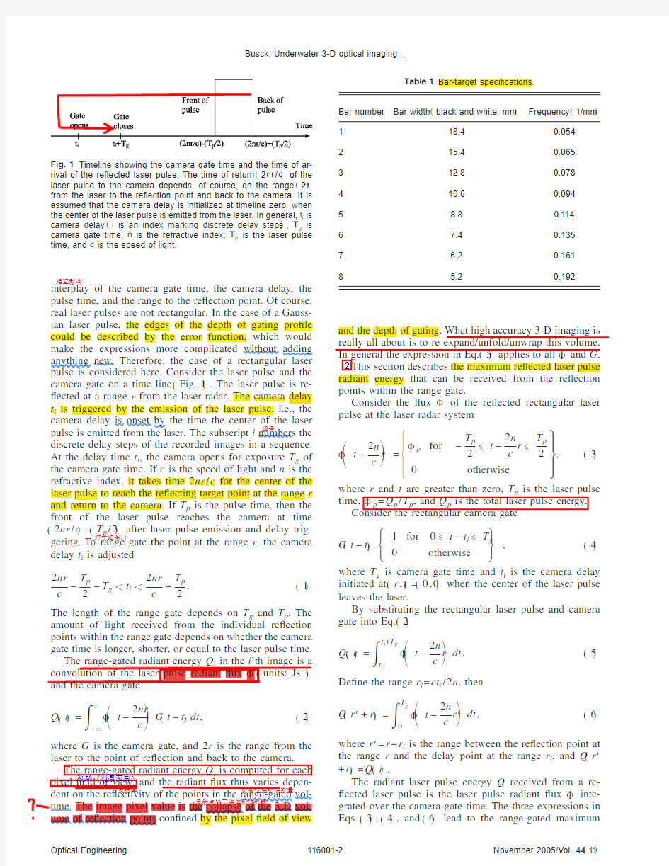
interplay of the camera gate time,the camera delay,the pulse time,and the range to the re?ection point.Of course,real laser pulses
are not rectangular.In the case of a Gauss-ian laser pulse,the edges of the depth of gating pro?le could be described by the error function,which would make the expressions more complicated without adding anything new.Therefore,the case of a rectangular laser pulse is considered here.Consider the laser pulse and the camera gate on a time line ?Fig.1?.The laser pulse is re-?ected at a range r from the laser radar.The camera delay t i is triggered by the emission of the laser pulse,i.e.,the camera delay is onset by the time the center of
the laser
pulse is emitted from the laser.The subscript i numbers the discrete
delay steps of the recorded images in
a sequence.At the delay time t i ,the camera opens for exposure T g of the camera gate time.If c is the speed of light and n is the refractive index,it takes time 2nr /c for the center of the laser pulse to reach the re?ecting target point at the range r and return to the camera.If T p is the pulse time,then the front of the laser pulse reaches the camera at time ?2nr /c ???T p /2?after laser pulse emission and delay trig-gering.To range gate the point at the range r ,the camera delay t i is adjusted
2nr c ?T p
2?T g ?t i ?2nr c +T p 2
.?1?
The length of the range gate depends on T g and T p .The amount of light received from the individual re?ection points within the range gate depends on whether the camera gate time is longer,shorter,or equal to the laser pulse time.Q i ?r ?=???
???
t ?
2nr
c ?
G ?t ?t i ?dt ,?2?
where G is the camera gate,and 2r is the range from the laser to the point of re?ection and back to the camera.The range-gated radiant energy Q i is computed for each pixel ?eld of view,and the radiant ?ux thus varies depen-is and the depth of gating.What high accuracy 3-D imaging is
really all about is to re-expand/unfold/unwrap this volume.In general the expression in Eq.?5?applies to all ?and G .This section describes the maximum re?ected laser pulse radiant energy that can be received from the re?ection points within the range gate.
Consider the ?ux ?of the re?ected rectangular laser pulse at the laser radar system ??
t ?2n
c
r ?
=
?
?p for ?
T p 2?t ?2n c r ?T p
20
otherwise
?
,?3?
where r and t are greater than zero,T p is the laser pulse time,?p =Q p /T p ,and Q p is the total laser pulse energy.Consider the rectangular camera gate G ?t ?t i ?=
?
1for 0?t ?t i ?T g 0
otherwise
?
,?4?
where T g is camera gate time and t i is the camera delay
initiated at ?r ,t ?=?0,0?when the center of the laser pulse leaves the laser.
By substituting the rectangular laser pulse and camera gate into Eq.?2?Q i ?r ?=
?t i
t i +T g ??
t ?
2n
c
r ?
dt .?5?
De?ne the range r i =ct i /2n ,then Q ?r ?+r i ?=
?0
T g ??
t ?
2n
c
r ??
dt ,?6?
where r ?=r ?r i is the range between the re?ection point at the range r and the delay point at the range r i ,and Q ?r ?+r i ?=Q i ?r ?.
The radiant laser pulse energy Q received from a re-?ected laser pulse is the laser pulse radiant ?ux ?inte-grated over the camera gate time.The three expressions in Eqs.?3?,?4?,and ?6?lead to the range-gated maximum
Table 1Bar-target speci?cations.
Bar number Bar width ?black and white,mm ?
Frequency ?1/mm ?
118.40.0542
15.40.065312.80.078410.60.09458.80.11467.40.1357
6.20.1618
5.2
0.192
Fig.1Timeline showing the camera gate time and the time of ar-rival of the re?ected laser pulse.The time of return ?2nr /c ?of the laser pulse to the camera depends,of course,on the range ?2r ?from the laser to the re?ection point and back to the camera.It is assumed that the camera delay is initialized at timeline zero,when the center of the laser pulse is emitted from the laser.In general,t i is camera delay ?i is an index marking discrete delay steps ?,T g is camera gate time,n is the refractive index,T p is the laser pulse time,and c is the speed of light.
相互影响
编号
对于距离门
反射率距离选通脉冲数量
视场(观景范围)
2
radiant energy Q ,?Eqs.?7?,?8?,and ?9??which can be used in a simpli?ed gated-viewing laser radar image simulation,
for example.A graphical representation of the depth of gat-ing ?Eqs.?7?,?8?,and ?9??is given in Fig.2.The length of the range gate is ?c /2n ??T g +T p ?.Given a camera delay range r i =?c /2n ?t i ,a laser pulse time T p ,and a camera gate time T g ,the closest gated point from the laser radar system is r =r ?+r i =?c /2n ??t i ?T p /2?,independent of camera gate time.The farthest gated point is r =r ?+r i =?c /2n ??t i +T g +T p /2?,dependent on both the pulse time and the camera gate time.When camera gate T g is equal to the laser pulse time T p ,the two range-gated pro?les merge into a single pro?le ?Fig.2?.Q ?r ?+r i ?=
Q p T p ?2n c r ?+T p
2
?
,for ?
T p 2?2n c r ??T p 2
if
T g ?T p ,
?7?
for
?T p 2?2n
c r ???T p 2
+T g if
T g ?T p .
Q ?r ?+r i ?=Q p ,for T p 2?2n
c r ???T p 2
+T g if
T g ?T p ,
or
?8?
Q ?r ?+r i ?=Q p
?T g
T p
?
,for ?
T p 2+T g ?2n c r ??T p
2
if
T g ?T p .
Q ?r ?+r i ?=?
Q p T p ?
2n c r ??T p
2
?T g ?
,for ?
T p
2+T g ?2n c r ??T p 2
+T g if
T g ?T p ,
?9?
for
T p 2?2n c r ??T p 2
+T g if
T g ?T p .
Otherwise Q ?r ?+r i ?=0.
When the camera gate T g is equal to the pulse time T p ,then Eq.?8?vanishes and Eqs.?7?and ?9?simplify.
In the following section,we propose a dynamic way of measuring the depth of gating pro?le.
3Dynamic Measurement of Depth of Gating
He and Seet have used a static method involving a station-ary set of bar targets to measure the depth of gating ?DOG ?.
They sample the DOG by placing bar targets along the range axis.A novel and dynamic method
is proposed here.Instead of spatial sampling,we sample the DOG in time.The camera delay is increased in steps of 0.1ns,which
gives about 10to 15sample points with a camera gate time
0.5ns and a laser pulse time 0.5ns.This is in close corre-spondence with the solution for the depth of gating for a rectangular laser pulse,which gives ten samples.The ex-periment gives a number of samples higher than ten be-cause the laser pulse is not rectangular,but more rounded with a fading tail.For the ?rst time,we present underwater optical 3-D images by computing the weighted average of the depth of gating DOG pro?le.A sequence of range gated 2-D images is recorded at 50Hz.Because of the simple relation between space and time of ?ight,the pixel values in the image sequence all represent the depth of gating.The individual pixel DOG curves are shifted compared to one another dependent on the range to the exact point of re?ec-the width of the DOG pro?le depends on the camera gate time.This is an important feature leading to the range correction discussed in Sec.5.The amplitude of the DOG pro?les increases with increasing camera gate time.This is partly explained by the shape of real laser pulses and partly by the camera gate time.
Fig.2Graphical representation of the exact solution of the depth of
gating ?DOG ?pro?le.Time and range are easily interchanged by multiplication of the speed of light.Top:The camera gate time T g is assumed longer than the rectangular laser pulse time T p .The x axis is a timeline marking the return of the laser pulse ?e.g.,by de?nition the front of the rectangular laser pulse reaches the camera at time 2nr ?/c =?T p /2?.The y axis is just the signal gated by the camera.Bottom:The camera gate time is assumed shorter than the laser pulse.Note that some of the laser pulse energy is wasted and only a fraction ?i.e.,Q p T g /T p ?is recorded by the camera.All the variables are de?ned in the text.?Note,Fig.1helps understand this ?gure.?
图示
进门卷积出门卷积
在近景上近距离通信的解决方案
4Experimental Setup
The principle of laser-pulse range gating is to keep the camera closed and wait until the re?ected photons from the target return to the camera.The laser pulse is emitted by the laser.When the laser pulse is emitted,the trigger pulse from the laser to the camera onsets the camera delay.The camera delay determines when the camera gate opens for recording the re?ected laser pulse.
The laser radar system consists of a pulsed laser and an
is a minor disadvantage and can be corrected by image processing or simply ignored.Figure 4shows the principle
of operation of the system.The camera gate time,delay,?cient.Figure 5shows a schematic diagram of the experi-mental setup.The setup is fairly simple with the laser radar system ?laser and CCD camera ?shooting directly into a 6-m-long water tube 40cm in diameter with a glass win-dow ?tted in one end.The target is placed in the tube through 25-cm-wide holes at the top of the tube.The output frames from the camera are sent to the computer.The laser radar system can either run in real-time gated viewing video mode or in 3-D image mode.
5Underwater Gated Viewing Imaging
The contrast of underwater objects/bottom decreases over time.If,for example,a sea mine is placed on the bottom,it will sooner or later be covered by silt,sediment,sand,
and/or micro-and macroscopic marine life.The objective quality of a 2-D image is very dependent on the image contrast.A zero contrast image is uniform and contains a minimum of information.However,the 3-D imaging tech-nique presented here proves that it can be applied in very low and zero contrast conditions.One of the strengths of the technique is that if the contrast is high,it can be wrapped onto the 3-D image,adding further information.Therefore,it is relevant to investigate the gated viewing contrast versus underwater range.Consider the contrast C =
A max ?A min
A max +A min
,
?10?
where A max and A min are the image maximum and minimum values.
A set of bar targets was applied underwater to determine the contrast.The contrast is determined by setting A max equal to the white bar value and A min equal to the black bar value.The widths of the bar targets are shown in Table 1.The bar targets are placed in the water tube and imaged with camera gate time 0.5ns.Figure 6shows the contrast measured at 3and 4m in tap water,and 4and 5m in sea water ?salinity of 15‰was measured ?.It is seen that the contrast of the widest bar decreases 12to 13%per meter.Extrapolating that means the contrast has decreased to zero at 10-m range and conventional 2-D images become use-less.However,this result depends on the water type and its optical properties.Figure 7shows the contrast data plotted against the angular resolution.To get a high bar-target con-trast,the black bar value should be as low as possible and
Fig.3Depth of gating pro?les measured in a dynamic way by step-ping the camera delay across a white board target.The camera delay step is 0.1ns.The x axis is labeled image number,but can easily be converted into a time axis by multiplication of the delay step of 0.1ns.The width of the pro?le depends on the camera gate time T g =0.3,0.4...1.0ns.To increase the signal-to-noise ratio of the pro?les,averaging has been done.Note that each data point represents the collapse of the 3-D space of re?ection points bounded by the depth of the range gate and the pixel ?eld of view.
Fig.4Principle of operation of pulsed 3-D gated viewing laser radar system starting in the upper left corner.
Fig.5Sketch of experimental setup.1?laser;2?direct trigger from laser to camera;3?camera;4?water tube ?0.4m diameter ?;5?tar-get;6?computer for adjustment of camera setting and processing of 3-D images;7?optical ?ber;and 8?lens to control the ?eld of illumination.
束缚
视频模式
宏观的
the white bar value as high as possible.If the difference between the white and the black cannot be altered,then the contrast can be increased by decreasing the average of the white and the black bar values ?see Eq.?10??.?For addi-tional information on contrast measurement and
modulation transfer function measurement using bar targets,
see Refs.
digital sampling can also contribute to contrast reduction.Scattering causes the re?ected light from the white bar to leak into the black bar,reducing the contrast.However,this effect is reduced by the short camera gate of 500ps.The contrast is mea-sured under the same conditions as the gated viewing 2-and 3-D laser radar imaging.The water type,the laser radar system settings,and the range are the same,i.e.,for each
3-D recording,the contrast has also been recorded.Scatter-ing is the major source of contrast reduction,and at longer
distances both scattering and absorption reduce the contrast
by attenuation.For a given range and bar-target period,the contrast depends on the turbidity of the water.It is experi-mentally veri?ed that ?ne 3-D images can be recorded even in low or zero contrast conditions.
The image technique applied here is that of For simplicity,consider the 1-D case.i image pixel value in the i ’th image in a sequence of range gated images,where the cam-era delay is increased in steps ?t .The computed range to the re?ection point ?r ?=c
2n
?
t 0+?t
?i
i ?I i ?i I i ?
,?11?
where c is the speed of light,n is the refractive index,t 0is
the camera delay,and ?t is the delay step.Equation ?11?states that the computed range to the re?ection point is the sampled and weighted average of the depth of gating pro-?le,which is sampled by stepping the camera delay across the re?ection point.To improve the range precision to the target,it is neces-sary to apply a novel linear correction for camera gate time.The range correction becomes evident when studying the exact solution of the depth of gating and the measured DOG pro?les,which are dependent on camera gate time.Consider the weighted image number ?i ?=?i
i ?I i ?i I i ,?12?where I i is the image value in the i ’th image.From the solution of the depth of gating,it follows ?set-ting I =Q ?t 0+?i ??t +
T g 2=2nr c ,?13?where t 0is the initial camera delay,?t is the delay step,T g is the camera gate time,and r is the range to the re?ection point.
According to Eqs.?11?,?12?,and ?13?,the weighted av-erage range is calculated by
Fig.6Underwater bar-target contrast versus bar frequency at 3and 4m in tap water and 4and 5m in sea water.At the lowest bar frequency,the contrast decreases roughly 12to 13%per meter of water.At long ranges and high frequencies,the contrast goes to zero.
Fig.7Underwater bar-target contrast versus angular resolution ?bar period/range ?.
水型
已证实的精细
?r ?=
c 2n ?t 0+?i ??t ?=r ?cT g 4n
,?14?
where the last equality is by substitution.Thus,the average range is corrected by an additional 5.64cm/ns to get the ?true ?range,assuming the water refractive index n =1.33.For example,with a gate time T g =0.5ns,the range correc-tion is 0.5ns ?5.64cm/ns=2.82cm.
Figure 8shows the target,which has been camou?aged by a layer of sand and placed on a sandy background.The shape of the target is suggested as a standard ?among oth-ers ?for evaluation of 3-D laser radar systems.The contrast of the target is low,even at 1-m range in air.By extrapola-tion of the contrast data ?Fig.6?,the contrast of the cam-ou?aged target is effectively zero at 4-and 5-m range in both sea and tap water.Figures 9,10,and 11show for the
?rst time the corrected 3-D images of the target at 4-and 5-m range in sea water ?Figs.9and 10?and 4m in tap water ?Fig.11?recorded with camera gate time 0.5ns and delay step 0.1ns.In general,the target is well preserved,though it has sunk a little into the background.The noise in the 3-D images arises from noise in the DOG pro?https://www.wendangku.net/doc/2111800246.html,paring Figs.9and 10,it is seen that 3-D image noise gets worse with range.This is explained by a decrease in signal-to-noise ratio ?SNR ?with range.The effect of tur-bidity on image quality and range computation is a de-crease in SNR,leading to a deterioration of the range ac-curacy.The range accuracy dependence on SNR has
been
Fig.8Target camou?aged by sand and placed on a sandy back-ground,thus providing a very low target/background contrast.Di-mensions:height 5cm,top diameter 6cm,and bottom diameter 12
cm.
Fig.93-D underwater gated viewing image of camou?aged target at 4-m range in sea water.Camera gate time is 500ps and delay step is 100ps.All axes are in
meters.Fig.103-D underwater gated viewing image of camou?aged target
at 5-m range in sea water.Camera gate time is 500ps and delay step is https://www.wendangku.net/doc/2111800246.html,pared to Fig.9,the range noise has increased from 4to 5m.This is explained by a decrease in signal-to-noise ratio ?SNR ?in the sequence of range gated images,and therefore a decrease in SNR of the DOG pro?les.All axes are in
meters.
Fig.113-D underwater gated viewing image of camou?aged target at 4-m range in tap water.Camera gate time is 500ps and delay step is 100ps.All axes are in meters.
discussed in a previous work.4In general,the point spread scattering effect of the water will round off the shape of the target.This is clearly seen in Figs.9,10,and11.The3-D images reveal the important fact that the applied method of gated viewing performs well beyond the limit where con-ventional2-D imaging breaks down.This is explained by the difference in recording techniques,where conventional imaging only uses the amplitude of the re?ected intensity, while gated viewing can combine intensity and the speed of light to created the3-D image.The3-D image processing time is only15to30s on a standard laptop?2.4GHz?, dependent on the number of images in the image sequence. The potential for high accuracy imaging in air has recently been proposed.4
6Summary and Conclusion
For the?rst time,an exact solution of the depth of gating ?DOG?of a gated viewing laser radar system is presented. The assumption of a rectangular laser pulse is far from the real shape of laser pulses,but nevertheless,the solution becomes simpler and the information gained about the lo-cation of the re?ection points within the depth of the range gate is of crucial importance for further development of 3-D gated viewing systems.Thus,a range correction of 5.64cm/ns for high accuracy3-D underwater gated view-ing imaging has been proposed.High accuracy and novel underwater3-D gated viewing images have been recorded in low and close to zero contrast conditions.By experi-ment,it is concluded that underwater contrast decreases with range,but it is not a limiting factor for gated viewing 3-D imaging,which is limited by attenuation,absorption, and scattering.
If the contrast is high enough,then a2-D underwater imaging mode for sea mine identi?cation is feasible.If the contrast is low,a3-D underwater imaging mode for sea nine identi?cation is feasible.Thus,the Navy’s sea mine identi?cation operator would need a switching capability between high contrast2-D gated viewing laser radar live video imaging and low contrast gated viewing3-D laser radar imaging.It is concluded that underwater gated view-ing laser radar images are of such a high quality that further trials involving the Danish Navy will be done in the future. Future studies may also involve moving targets. Acknowledgments
The author would like to acknowledge Stig V.Platen,Hen-rik Fürst,Joachim F.Andersen,and Henning Heiselberg at the Danish Defence Research Establishment for their help.References
1.G.R.Fournier,D.Bonnier,J.L.Forand,and P.W.Pace,“Range-
gated underwater laser imaging system,”Opt.Eng.329,2185–2190?1993?.
2.O.Steinvall,L.Klasen,T.Chevalier,P.Andersson,https://www.wendangku.net/doc/2111800246.html,rsson,M.
Elmqvist,and M.Henriksson,“Grindad avbildning—fordjupad studie,”?Gated viewing—preliminary study?,FOI-R-0991-SE,Swed-ish Defence Research Agency,Link?bing,Sweden?2003?.
3.L.Klasen,P.Andersson,https://www.wendangku.net/doc/2111800246.html,rsson,T.Chevalier,and O.Steinvall,
“Aided target recognition from3-D laser radar data,”Proc.SPIE 5412,321–332?2004?.
4.J.Busck and H.Heiselberg,“Gated viewing and high-accuracy three-
dimensional laser radar,”Appl.Opt.43,4705–4710?2004?.
5. A.Nevis,R.J.Hilton,S.J.Taylor,B.Cordes,and J.W.McLean,
“The advantages of three-dimensional electro-optic imaging sensors,”
Proc.SPIE5089,225–237?2003?.
6. A.Nevis,“Automated processing for streak tube imaging lidar data,”
Proc.SPIE5089,119–129?2003?.
7. A.Gleckler and A.Gelbart,“Three-dimensional imaging polarime-
try,”Proc.SPIE4377,175–185?2001?.
8. A.D.Gleckler,“Multiple-slit streak tube imaging lidar?MS-STIL?
applications,”Proc.SPIE4035,266–278?2000?.
9.J.W.McLean and J.T.Murray,“Streak-tube lidar allows3-D ocean
surveillance,”Laser Focus World34?1?,171–176?1998?.
10.R.Stettner,H.Bailey,and R.Richmond,“Eye-safe laser radar3-D
imaging,”Proc.SPIE5412,111–116?2004?.
11. B.W.Schilling,D.N.Barr,G.C.Templeton,L.J.Mizerka,and C.
W.Trussell,“Multiple-return laser radar for three-dimensional imag-ing through obscurations,”Appl.Opt.41,2791–2799?2002?.
12.L.J.Mullen,https://www.wendangku.net/doc/2111800246.html,ux,B.Concannon,E.P.Zege,I.L.Katsev,and A.
S.Prikhach,“Amplitude-modulated laser imager,”Appl.Opt.43, 3874–3892?2004?.
13. F.Pellen.,P.Olivard,Y.Guern,J.Cariou,and J.Lotrian,“Radio-
frequency modulation on optical carrier for target detection enhance-ment in seawater,”Proc.SPIE4488,13–24?2002?.
14. B.Redman,W.C.Ruff,and K.Aliberti,“Direct detection laser vi-
brometry with an amplitude modulated ladar,”Proc.SPIE5412, 218–228?2004?.
15. B.A.Swartz and J.D.Cummings,“Laser range-gated underwater
imaging including polarization discrimination,”Proc.SPIE1537, 42–56?1991?.
16. E.A.McLean,H.R.Burris,and M.P.Strand,“Short-pulse range-
gated optical imaging in turbid water,”Appl.Opt.34,4343–4351?1995?.
17. D.M.He and G.G.L.Seet,“Underwater lidar imaging scaled by
22.5cm/ns with serial targets,”Opt.Eng.433,754–766?2004?. 18. D.M.He and G.G.L.Seet,“Underwater lidar imaging in highly
turbid waters,”Proc.SPIE4488,71–81?2002?.
19.G.D.Boremann and S.Yang,“Modulation transfer function mea-
surement using three-and four-bar targets,”Appl.Opt.34,8050–8052?1995?.
20. D.N.Sitter,J.S.Goddard,and R.K.Ferrell,“Method for the modu-
lation transfer function of sampled imaging systems from bar-target patterns,”Appl.Opt.34,746–751?1995?.
Jens Busck received his BSc and MSc degrees in geophysics from the University of Copenhagen,Denmark,in1999and2001,respec-tively.In2005he?nished his PhD about3-D laser radar experi-ments and simulation in the atmosphere and underwater,from the Danish Defense Research Establishment and Technical University of Denmark.His current research interests include laser radar sys-tems,2-and3-D imaging,underwater turbulence,and remote sens-ing in general.
质心算法代码
clear all,clc; for n=6:2:14 x=100*rand(1,100); %布置10m*10m的网格区域y=100*rand(1,100); w=100*rand(1,n); z=100*rand(1,n); plot(x,y,'b*',w,z,'rO') axis([0 100 0 100]) grid on; xlabel('x'),ylabel('y') title('原始点分布') C=0; X=zeros(1,100); Y=zeros(1,100); for i=1:100 m=0; a=0; b=0; for k=1:n dist=distance(x(i),y(i),w(k),z(k)); if dist<=2 a=a+w(k); b=b+z(k); m=m+1; end end if m>=1 X(i)=a/m; Y(i)=b/m; else X(i)=0; Y(i)=0; C=C+1 ; end end % plot(X,Y,'bO') axis([0 10 0 10]) grid on; xlabel('x'),ylabel('y') title('定位后点分布') ALE=0; for i=1:100
ALE=ALE+sqrt((X(i)-x(i))^2+(Y(i)-y(i))^2); end ALE=ALE/100; ALE=ALE/4; c1(n/2-2)=(100-C)/100 ale1(n/2-2)=ALE bili(n/2-2)=n/(100+n); end figure ; plot(bili,c1); grid on; xlabel('锚节点比例'),ylabel('可定位节点比例') title('锚节点比例与可定位节点比例图'); figure, plot(bili,ale1); xlabel('锚节点比例'),ylabel('定位误差') grid on; title('锚节点比例与定位误差')
N维空间几何体质心的计算方法.
N维空间几何体质心的计算方法 摘要:本文主要是求一个图形或物体的质心坐标的问题,通过微积分方面的知识来求解,从平面推广到空间,问题也由易到难。首先提出质心或形心问题,然后给出重心的定义,再由具体的例子来求解相关问题。 关键字:质心重心坐标平面薄板二重积分三重积分 一.质心或形心问题: 这类问题的核心是静力矩的计算原理。 1.均匀线密度为M的曲线形体的静力矩与质心: 静力矩的微元关系为 , dMx yudl dMy xudl ==. 其中形如曲线L( (, y f x a x b =≤≤的形状体对x轴与y轴的静力矩分别 为( b
a y f x S = ? , ( b y a M u f x =? 设曲线AB L 的质心坐标为( ,x y,则,, y x M M x y
M M == 其 中( b a M u x d x u l == ? 为AB L 的质量,L为曲线弧长。若在式 y M x M
= 与式 x M y M = 两端同乘以2π,则可得 到22( b a y xl f x S ππ == ? ,
22( b a x yl f x S ππ == ? ,其中x S 与y S 分别表示曲线AB L 绕x轴与y轴旋转而成的旋转体的侧面积。 2.均匀密度平面薄板的静力矩与质心: 设f(x为 [],a b 上的连续非负函数,考虑形如区域 {} (,,0(
D x y a x b y f x =≤≤≤≤ 的薄板质心,设M为其密度,利用微元法,小曲边梯形MNPQ的形心坐标为1 (,(, 2 y f y x y x x ≤≤+? ,当分割无限细化时,可当小曲边梯形MNPQ的质量视为集中于点 1 (,( 2 x f x 处的一个质点,将它对x轴与y轴分别取静力矩微元可有 1 (( 2 x dM u f x f x dx
汽车质心位置的计算.qicheban
汽车质心位置的计算 燕山大学 车辆与能源学院 裴永生 2011年12月7日
汽车质心位置的计算 1、 质心到前轴(坐标原点)的水平距离 (1) 常规公式: gi Xi gi a ∑?∑=)( ------------------------(1) 式中 a 质心到前轴的水平距离 gi 各总成(或载荷)质量 Xi 各总成(或载荷)到前轴的水平距离 轴荷(或簧载质量): gi L a G ∑?-=)1(1 L Xi gi gi )(?∑-∑= ------------------------(2) gi L a G ∑?= 2 L Xi gi )(?∑= ------------------------(3) 式中 1G 前轴负荷(或前簧载质量) 2G 后轴负荷(或后簧载质量) L 轴距 (2) 先求轴荷再算质心位置: ?? ?????-∑=gi L Xi G )1(1
------------------------(2a ) ???????∑=gi L Xi G 2 ------------------------(3a ) )1(12G G L G G L a -?=?= ------------------------(4) 式中 gi G G G ∑=+=21 总负荷(或簧载总质量) 2、 质心离地高度 常规公式: gi hi gi h ∑?∑=)( -------------------------(5) 式中 h 质心到地面的高度 hi 各总成(或载荷)离地高度 *注:可以先算出)(hi gi ?∑再除以gi ∑,也可以先算出)( gi hi gi ∑?再合成。 3、 各种质心的分别计算和合成 (1) 分别计算: ① 空载、满载状态的质心位置
质心算法
3.1 质心检测算法 系统采用质心法进行数据处理能提高测试精度。因为质心法能使CCD 上的图像分辨率达到光敏元尺寸的1/10,那么成像亮线中心在CCD 上所对应的光敏源序号就可以是小数,而非一定是整数,这样通过计算可知,精度提高了0.1个百分点。虽然测量系统的精度有提高,但0.11%的相对误差仍不能令人满意,从误差公式可知,系统误差的改善主要取决于CCD 的像元尺寸。随着CCD 技术的不断发,像元尺寸也会不断改善,系统误差也将会有大幅度减小。 质心法图像预处理算法步骤如下[5]:(1)对图像通过灰度化和反色后阈值选择得到光斑特征区域;(2)模糊去噪(mean blur ),消除热噪声以及像素不均匀产生的噪声;(3)再次进行阈值选择,得到更清晰的光斑区域;(4)形态学处理,选择disk 中和合适的领域模板,对图像进行腐蚀和填充处理,以得到连通域的规则形状图形;(5)边缘检测得到图像边缘,反复实验证明canny 边缘检测算法最好;(6)对边缘再进行形态学strel -imerode -imclose -imfill 相关运算得到更连通的边缘曲线,调用regionprops (L ,properties )函数,根据质心法计算质心。 下面介绍几种常用的质心算法 (1)普通质心算法 (,)ij ij ij c c ij ij x I x y I =∑∑ (3-1) 其中ij I 为二维图像上每个像素点所接收到的光强,该算法适用于没有背景噪 声,背景噪声一致或信噪比较高的情况。 (2)强加权质心算法 0000000000000000,/2,/2 ,/2,/2 ,/2,/2 ,/2,/2y w y x w x i ij j y w y i x w x c y w y x w x ij j y w y i x w x x I w x I w ++=-=-++=-=-=∑∑∑∑
汽车质心位置的计算
汽车质心位置的计算 1、 质心到前轴(坐标原点)的水平距离 (1) 常规公式: gi Xi gi a ∑?∑=)( ------------------------(1) 式中 a 质心到前轴的水平距离 gi 各总成(或载荷)质量 Xi 各总成(或载荷)到前轴的水平距离 轴荷(或簧载质量): gi L a G ∑?-=)1(1 L Xi gi gi )(?∑- ∑= ------------------------(2) gi L a G ∑?=2. L Xi gi )(?∑= ------------------------(3) 式中 1G 前轴负荷(或前簧载质量) 2G 后轴负荷(或后簧载质量) L 轴距 (2) 先求轴荷再算质心位置: ????? ??-∑=gi L Xi G )1(1 ------------------------(2a ) ?? ?????∑=gi L Xi G 2 ------------------------(3a )
)1(12G G L G G L a -?=?= ------------------------(4) 式中 gi G G G ∑=+=21 总负荷(或簧载总质量) 2、 质心离地高度 常规公式: gi hi gi h ∑?∑=)( -------------------------(5) 式中 h 质心到地面的高度 hi 各总成(或载荷)离地高度 *注:可以先算出)(hi gi ?∑再除以gi ∑,也可以先算出)( gi hi gi ∑?再合成。 3、 各种质心的分别计算和合成 (1) 分别计算: ① 空载、满载状态的质心位置 空载: gi 不包括乘员或/和载荷,仅包括相关总成。 满载: gi 包括乘员或/和载荷以及相关总成。 ② 簧载质量、非簧载质量的质心位置 簧载质量:gi 只包括属于簧载质量的总成,或者还包括乘员或载荷。 非簧载质量:gi 只包括属于非簧载质量的总成。
光电雷达-距离选通技术
距离选通激光雷达技术 摘要:成像激光雷达无论在军用领域还是民用领域日益得到广泛的应用。其中,激光距离选通成像技术经过数十年的发展,在军事侦察、搜救、监视、水下探测等方面获得重要的应用。本文介绍了距离选通激光雷达的工作原理,对距离选通激光雷达设计中的关健技术进行分析,给出了几种具备代表性的元件及其指标。 关键词:激光雷达;同步控制;距离选通;主动成像 引言 1960 年世界上第一台激光器诞生以来,激光雷达便以其独特的优势成为雷达研究领域的热门项目,其中无扫描成像是激光雷达发展趋势之一[1]。 一般的成像激光雷达在对水中的目标进行成像探测时,或者陆地探测而大气中含有较多的雨、雾或烟等悬浮颗粒时,就会产生很强的前向和后向散射,又或者在海上、雪地或者白天等环境中探测时,会产生很强的背景光辐射,这些情况都会对成像质量造成严重影响。为了使激光雷达能在上述情况中也能够很好的工作,人们发明了距离选通技术,并且逐步成为人们研究的热点[2]。 距离选通激光雷达能很好的消除背景光及散射的影响,在上述复杂环境中获得目标的 2D强度像,并且经过进一步的数据处理还可以从多幅的 2D像中获得关于距离的 3D距离像[3]。距离选通激光成像激光雷达系统属于主动成像,它不仅可以克服被动成像的一些缺点,比如能够获得更高的成像分辨率,不受环境的背景光的影响等;而且同时它也可以弥补主动成像的一些不足,降低大气散射、湍流等对激光脉冲的前行波和回波的影响,使其在水底目标成像和矿产探测,远距离军事目标识别和跟踪方面都可以有很广泛应用[4]。 1 成像激光雷达 近年来人们对成像激光雷达的研究越来越关注,并且成像激光雷达有着取代传统微波雷达的趋势[5]。这是因为激光成像雷达有着微波雷达无法比拟的优
三维激光成像
激光测距系统是复合光电系统的一个重要单元,将激光测距技术与摄影测量技术相结合,实现三维激光成像,对提高目标识别准确性和观测能力有重要意义。请尽快确定课题完成方式,完善相关技术路线,开展课题调研论证工作。80 三维激光成像 根据有无照明光源,成像系统可以分为主动成像系统和被动成像系统两种。被动成像系统最大的特点就是本身不带光源,依赖于环境或目标的发光,容易受到环境光源的影响。主动成像系统采用一个人造光学辐射源(一般为激光器)和接收器,其接收器用于收集和探测目标景物直接或反射的部分光辐射,具有成像清晰、对比度高,不受坏境光源的影响等优点。 激光由于它有亮度高、单色性和方向性好三个方面的优点,是人们早就渴望得到的理想的测距光源,因此在它出现后不到一年的时间就被用于测距。激光测距系统是复合光电系统的一个重要单元,它虽然经过了多代的更新和变化,且型号繁多,诸如激光测月系统、火炮激光测距系统、测地激光测距系统、测距光雷达等系统,但无论怎么变,其基本原理和技术还是大同小异。 一.激光测距分类 随着激光测距的广泛应用和不断发展,测距系统的种类也愈来愈多样化。按照激光测距的原理区分,大体有如下三类。 1.脉冲测距法 在测距点向被测目标发射一束短而强的激光脉冲,光脉冲发射到目标上后其中一小部分激光反射到测距点被光功能接受器所接收。假定光脉冲在发射点与目标间来回一次所经历的时间间隔为t ,那么被测目标的距离R 为: 2ct R = (1) 式中,c 为光速。 当认为光速一定时(不考虑大气中光速的微小变化),测距精度 2t c R ?=? (2) 2.相位测距法 相位法是通过测量单色连续激光的调制波在待测距离上往返传播所发生的相位变化,间接测量时间t 2D 。来计算距离D )2/)(2/()2/(2f c t c D D πΦ== (3) 式中:c 为光速在空气中传播的速度,Ф为调制光信号经过被测距离D 而产生的相位移,f 为信号的调制频率。
质心定位算法 江南大学
无线传感网技术实验报告(三) 班级:微电子1101学号:0301110115姓名:杨海平 一,实验目的: 通过仿真实验掌握无线传感器网络的定位算法—质心定位算法。 二,实验内容: 在100*100M2的正方形区域里,有n个信标节点和一个未知节点,未知节点和新表节点的通信半径均为R,则: (1),当通信半径R=50M,信标节点个数n=6,12,18,24,30时,利用Monte Carlo方法,分别计算未知节点的实际位置与估计未知的平均误差; (2),当信标节点个数n=20,通信半径R=5,10,15,20,25,30,35,40,45,50m时,利用Monte Carlo方法,分别计算未知节点的实际位置与估计位置的平均误差; 三,实验方法: (1),在边长为100m的正方形中,产生一个信标节点为n,未知节点为1的随机分布图; (2),确定与未知节点相连的信标节点; (3),利用质心算法,对未知节点的位置进行估计; (4),每一组数据(信标节点个数n,通信半径R)需要仿真800次,得出该组数据下未知节点的实际位置与估计位置的平均误差。 四,实验分析过程: (1),实验内容一:当通信半径R=50M,信标节点个数n=6,12,18,24,30时,按照实验一的方法随机产生X,Y坐标为0~100的n个信标节点的坐标,再随机产生一个未知节点的X,Y坐标,然后判断n个信标节点是否能与未知节点通信,把能与未知节点通信的信标节点X,Y坐标相加,除以能与未知节点通信的节点数,即为用质心定位算法估计的未知节点个数,误差即为未知节点与估计未知节点坐标的距离。每组信标节点个数仿真800次,累加每次仿真的误差,取平均值即得到估计误差。 (2),实验内容二:思想方法与实验内容一相同,当信标节点个数n=20,通信半径R=5,10,15,20,25,30,35,40,45,50m时,每组通信半径仿真800次,累加每次仿真的误差,取平均值即得到估计误差。 五,程序 (1),实验内容一程序如下: clear all; close all; nbeacon=[612182430];%信标节点个数n=6,12,18,24,30 nbeaconi=5; error=zeros(1,nbeaconi);%误差数组error nunknow=1;%知节点个数为1 r=50;%通信半径r为50 optimes=800; for ni=1:1:5;%每组信标节点得到一个平均误差 errorsum=0; validtimes=0;%800次仿真中至少有一个信标与未知节点通信的次数 for optimei=1:1:optimes
N维空间几何体质心的计算方法
N维空间几何体质心的计算方法 摘要:本文主要是求一个图形或物体的质心坐标的问题,通过微积分方面的知识来求解,从平面推广到空间,问题也由易到难。首先提出质心或形心问题,然后给出重心的定义,再由具体的例子来求解相关问题。 关键字:质心重心坐标平面薄板二重积分三重积分 一.质心或形心问题: 这类问题的核心是静力矩的计算原理。 1.均匀线密度为M的曲线形体的静力矩与质心: 静力矩的微元关系为 , dMx yudl dMy xudl ==. 其中形如曲线L( (), y f x a x b =≤≤)的形状体对x轴与y轴的静力矩分别 为( b a y f x S = ? , ( b y a M u f x =? 设曲线AB L 的质心坐标为( ,x y),则,, y x M M x y M M == 其 中() b a M u x d x u l == ? 为AB L 的质量,L为曲线弧长。 若在式 y M x M = 与式 x M y M = 两端同乘以2π,则可得 到22() b a y xl f x S ππ == ? , 22( b a x yl f x S ππ == ? ,其中x S 与y S 分别表示曲线AB L 绕x轴与y轴旋转而成的旋转体的侧面积。 2.均匀密度平面薄板的静力矩与质心: 设f(x)为 [],a b 上的连续非负函数,考虑形如区域 {} (,),0() D x y a x b y f x =≤≤≤≤ 的薄板质心,设M为其密度,利用微元法,小曲边梯形MNPQ的形心坐标为 1 (,()), 2 y f y x y x x ≤≤+? ,当分割无限细化时,可当小曲边梯形MNPQ的质量视为集中于点 1 (,()) 2 x f x 处的一个质点,将它对x轴与y轴分别取静力矩微元可有 1 ()() 2 x dM u f x f x dx = , () y dM uxf x dx = .两个静力矩为2 1 () 2 b x a M u f x dx =? ? , () b x a M u xf x dx =?.设质心坐标为(,) x y,则有() y b a M u x xf x dx M M ==? , 2 1 () 2 y b a M u y f x dx M M ==? .其中 () b a M u f x dx MA == ? 为该
整车计算及质心位置确定
第六章整车计算及质心位置确定 第一节轴荷计算及质心位置确定 1、本章所用质量参数说明(Kg) T 底盘承载质量 F 底盘整备质量(不含上车装置) NL 有效载荷 V A1 底盘整备质量时的前轴荷 HA1 底盘整备质量时的后轴荷 V A2 允许前轴荷 HA2 允许后轴荷 HAG2 允许总的后轴荷(驱动轴+支撑轴) NLA2 允许后支撑轴轴荷 VLA2 允许中支撑轴轴荷 GG2 允许总质量(载货汽车底盘整备质量+上车装置质量+允许载荷) NL2 允许有效载荷 V A3 实际有效载荷(AB+NL)时的前轴荷 HA3 实际有效载荷(AB+NL)时的后轴荷) GG3 实际有效载荷(AB+NL)时的总质量 NL3 实际有效载荷(AB+NL) HA4 底盘后轴荷(包括所有附加质量例如驾驶员、附加油箱,但不含AB和NL)GG4 底盘总质量(包括所有附加质量例如驾驶员、附加油箱,但不含AB和NL)NLV 由轴荷超载引起的有效载荷损失 HAü超过允许后轴荷 V Aü超过允许前轴荷 AB 上车装置质量 EG整车整备质量(载货汽车底盘+AB) M 附加质量,例如: M1 驾驶员+副驾驶员 M2 备胎(新、老位置移动时) M3 起重机(随车吊)、起重尾板等 LV A 前轴荷占总质量的比例(%) 2、本章所用尺寸参数说明(mm) A、轴距
A1、轴距(第一后轴中心线至第二后轴中心线) A理论理论轴距(只用于3轴或4轴) a1 与轴荷比例(驱动轴与支撑轴之比)有关的从理论轴线到驱动轴的距离W 前轴中心线至驾驶室后围的距离 W2 前轴中心线至上车装置前缘的距离 X 货厢或上车装置的长度 y 均布载荷时最佳质心位置至前轴中心线的距离(AB+NL) y'假设的质心位置至前周中心线的位置 y1 驾驶员+副驾驶员位置距前轴中心线位置 y2 备胎(新、老位置移动的距离) y3 起重机(随车吊)、起重尾板等 MHS 附加质量的质心高度 GHSL 整车空载质心高度 GHSV 整车满载质心高度 FHS 底盘的质心高度 ABHS 上车装置的质心高度 NLHS 允许有效载荷的质心高度 2、轴荷计算 a)双后轴: a1=A1/2 A理论=A+a1 b)后支撑轴: a1=NLA2×A1/HAG2
物体质心计算方法
物体质心计算方法 卢庆杨晓赟 摘要叙述了通过用圆规和直尺画出重物质心位置的方法及其原理分析。 关键词质心规尺作图载荷线段 1 前言 作为工程设计人员,计算零、部、组件及总成的质心是经常性的工作。虽然质心的计算方法多种多样,但计算工作量大,常常不得不经过反复验算后才能确定。下面以计算汽车质心为例,向大家介绍一种简单实用的计算质心的方法——规尺作图法。 2 水平方向质心 (即后轴载荷缩小K′倍,取K′=10);通过B点垂直于AB向下画一线段BD,其长度等于63.7 mm(即前轴载荷缩小K′倍)。 最后,连接C、D两点,与线段AB交于点O,该点即为汽车在水平方向上的质心,量出AO的长度乘以K(K=10)为847mm,即质心在在水平方向上距前轴的距离。 注:K、K′为任意实数,二者可以不相等。作图时,前轴载荷画在后轴上,后轴载荷画在前轴上,且二者必须位于线段AB的两侧。 3 原理分析 我们知道力是矢量,有大小和方向,可以用线段来表示。矢量三角形,就是我们最常见的例子。下面我们将把力用长度来表示。 本文中,如图1所示,在测水平方向质心时,是以汽车为研究对象,对质心G取矩,即有
M G=F A×L AO=F B×L BO (1)所以 L AO/L BO=F B/F A (2)式中: M G—对质心G的力矩; F A、F B—前、后轴载荷; L AO、L BO—质心距前、后轴距离。 由公式(2),我们可将求质心的问题简化为:已知F A、F B大小,及线段AB长度,求AB上一点O,使得AO/BO=F B/F A。 解题过程如下: (1) 如图3,画出已知线段AB; (2) 过A作AE⊥AB,取线段AC=F B, CE=F A; AB 图 3 原理分析图 B CE∥BD,CD∥BE,所以BD=CE=F A。 h=600mm,其前、后轴的 图4 抬高前轴测前、后轴载荷 如图5,BE与水平地面平行,E为A在BE上的投影,图中AE=60mm,CE=37.57mm,BD=60.43mm。连接CD,交BE于点O′,该点即为汽车质心G在BE上的投影。连接A、B两点,取AO=84.7mm。过点O作AB的垂线,与过O′的垂线(垂直于BE)交于点G,该点即为汽车的质心。线段GO即为汽车质心距车轴AB的距离(316mm),再加
matlab计算质心的程序
李娜理论物理1334080 第三次作业(1) >>A=[sqrt(3),0,0,0,0,0,0,2,0;... 1,2,0,0,0,0,0,0,0;... -1,0,1,2,0,0,0,0,0;... sqrt(3),0,sqrt(3),0,0,0,0,0,0;... 0,0,0,0,sqrt(3),0,sqrt(3),0,0;... 0,0,0,-2,-1,0,1,0,0;... 0,0,sqrt(3),0,sqrt(3),0,0,0,0;... 0,-2,-1,0,sqrt(3),2,0,0,0;... 0,0,0,0,0,0,sqrt(3),0,2]; >> b=[0;0;0;0;0;0;40;0;0]; >> x=A\b x = -11.5470 5.7735 11.5470 -11.5470 11.5470 1.5470 -11.5470 10.0000 10.0000
(2) function hj A=[sqrt(3),0,0,0,0,0,0,2,0;... 1,2,0,0,0,0,0,0,0;... -1,0,1,2,0,0,0,0,0;... sqrt(3),0,sqrt(3),0,0,0,0,0,0;... 0,0,0,0,sqrt(3),0,sqrt(3),0,0;... 0,0,0,-2,-1,0,1,0,0;... 0,0,sqrt(3),0,sqrt(3),0,0,0,0;... 0,-2,-1,0,sqrt(3),2,0,0,0;... 0,0,0,0,0,0,sqrt(3),0,2]; b=[0;0;0;0;0;0;40;0;0]; x=A\b; while abs(max(x(1:7)))<=100 b(7)=b(7)+0.1; x=A\b; end disp(b(7)/2) >> hj 173.2500
轴荷分配及质心位置的计算
4 轴荷分配及质心位置的计算 4.1轴荷分配及质心位置的计算 根据力矩平衡原理,按下列公式计算汽车各轴的负荷和汽车的质心位置: g 1l 1+g 2l 2+g 3l 3+…=G 2L g 1h 1+g 2h 2+g 3h 3+…=Gh g g 1+g 2+g 3+…=G (4.1) G 1+G 2=G G 1L=Gb G 2L=Ga 式中: g 1 、g 2、 g 3—— 各总成质量,kg ; l 1 、l 2 、l 3—— 各总成质心到前轴距离,m ; h 1 、h 2 、h 3—— 各总成质心到地面距离,m ; G 1—— 前轴负荷,kg ; G 2—— 后轴负荷,kg ; L —— 汽车轴距,m ; a ——汽车质心距前轴距离,m ; b ——汽车质心距后轴距离,m ; h g ——汽车质心到地面高度,m 。 质心确定如表 4.1所示 表4.1 各部件质心位置 部件 重量i g i l i h (满) i h (空) i gh i gh (满) i gh (空) 人 195 0 1.3 1.4 0 253.5 273 发动机附件 340 0.1 0.9 1 34 306 340 离合器及操纵机构 8.4 1 0.85 0.94 8.4 7.14 7.896
变速器及离合器壳 112 0.4 0.85 0.94 44.8 95.2 105.28 后轴及后轴制动器 260 3.36 0.17 0.82 873.6 44.2 213.2 后悬架及减振器 135 3.36 0.6 0.65 453.6 81 87.75 前悬架及减振器 40.5 0.6 0.72 24.3 29.16 前轴前制动器轮毂转向梯形 151.9 0 0.7 0.8 0 106.33 121.52 车轮及轮胎总成 310.6 2.3 0.6 0.65 714.38 186.36 201.89 车架及支架拖钩装置 263 2.6 0.7 0.8 683.8 184.1 210.4 转向器 16.9 -0.35 0.9 0.95 -5.915 15.21 16.055 挡泥板 64.5 1.6 0.6 0.7 103.2 38.7 45.15 油箱及油管 16.3 1.4 0.6 0.65 22.82 9.78 10.595 蓄电池组 33.8 1.4 0.6 0.65 47.32 20.28 21.97 车箱总成 317.3 2.7 0.9 1 856.71 285.57 317.3 驾驶室 179.8 0.2 1.1 1.2 35.96 197.78 215.76 货物 2250 2.85 1.2 6412.5 2700 0 ∑ 4695 10258.06 4555.45 2216.926 ⑴.水平静止时的轴荷分配及质心位置计算 根据表4.1所求数据和公式(4.1)可求 满载: G 2= kg L l g n i i i 99.305236 .310258.06 1 == ∑= G 1=4695-3052.99=1642.01kg m G L G a 18.24695 36 .399.30522=?=?= m a L b 18.118.236.3=-=-= 前轴荷分配: 4695 01 .16421=G G =35.0%