comsol电场示例

Computing the Effect of Fringing Fields on Capacitance

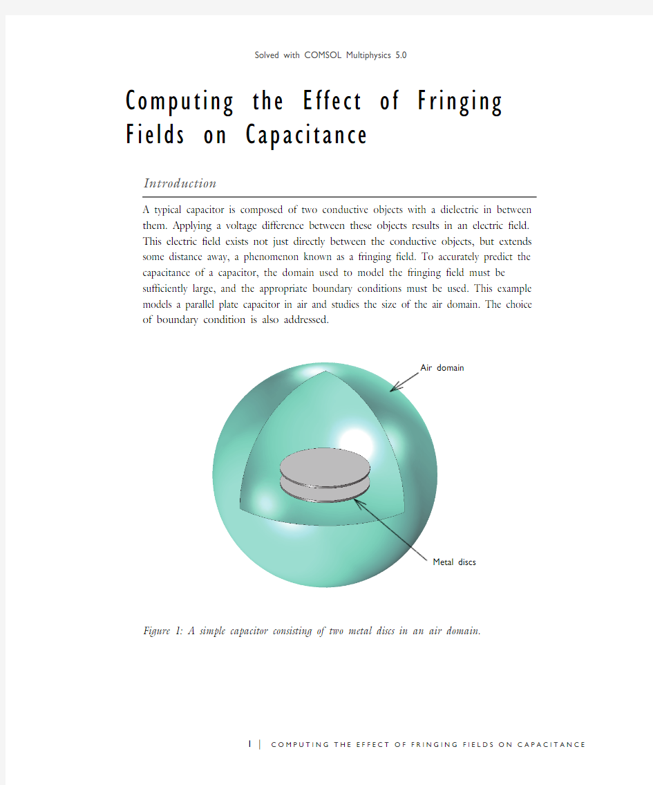
Introduction

A typical capacitor is composed of two conductive objects with a dielectric in between

them. Applying a voltage difference between these objects results in an electric field.

This electric field exists not just directly between the conductive objects, but extends some distance away, a phenomenon known as a fringing field. To accurately predict the capacitance of a capacitor, the domain used to model the fringing field must be

sufficiently large, and the appropriate boundary conditions must be used. This example models a parallel plate capacitor in air and studies the size of the air domain. The choice of boundary condition is also addressed.

Air domain

Metal discs Figure 1: A simple capacitor consisting of two metal discs in an air domain.

Model Definition

Figure 1 shows the capacitor consisting of two metal discs in a spherical volume of air. The size of the sphere truncates the modeling space. This model studies the size of this air domain and its effect upon the capacitance.

One of the plates is specified as ground, with a voltage of 0 V. The other plate has a specified voltage of 1 V. It is only the difference in the voltage between these plates that affects the capacitance and electric field strength; the voltage itself is arbitrary.

The air sphere boundary can be thought of as one of two different physical situations: It can be treated as a perfectly insulating surface, across which charge cannot redistribute itself, or as a perfectly conducting surface, over which the potential will not vary.

The modeling realization of the perfectly insulating surface is the Zero Charge boundary condition. This boundary condition also implies that the electric field lines are tangential to the boundary.

The modeling realization of the perfectly conducting surface is the Floating Potential boundary condition. This boundary condition fixes the voltage of all of the boundaries of the sphere to a constant, but unknown, value that is computed during the solution. The boundary condition also implies that the electric field lines are perpendicular to the boundary.

When studying convergence of results with respect to the surrounding domain size, it is important to fix the element size. In this model, the element size is fixed as the domain size is varied.

Results and Discussion

Figure 2 and Figure 3 plot the electric field for the cases where the air sphere boundary is treated as perfectly insulating and perfectly conducting, respectively. The fields terminate differently on the boundaries of the air sphere.

Figure 4 compares the capacitance values of the device with respect to air sphere radius for the two boundary conditions. The figure also plots the average of the two values. Notice that all three capacitance calculations converge to the same value as the radius grows. In practice, it is often sufficient to model a small air sphere with the electric insulation and floating potential boundary conditions and to take the average of the two.

Zero Charge boundary condition.

Floating Potential boundary condition.

Figure 4: Convergence of the device capacitance as the size of the surrounding air sphere is increased. Electric insulation and fixed voltage boundary conditions converge to the same result. The average of the two is also plotted.

Model Library path: ACDC_Module/Capacitive_Devices/

capacitor_fringing_fields

Modeling Instructions

From the File menu, choose New.

N E W

1In the New window, click Model Wizard.

M O D E L W I Z A R D

1In the Model Wizard window, click 3D.

2In the Select physics tree, select AC/DC>Electrostatics (es).

3Click Add.

4Click Study.

5In the Select study tree, select Preset Studies>Stationary.

6Click Done.

D E F I N I T I O N S

Parameters

1On the Model toolbar, click Parameters.

2In the Settings window for Parameters, locate the Parameters section.

3In the table, enter the following settings:

Name Expression Value Description

r_air15[cm]0.15000 m Radius, air domain

G E O M E T R Y1

1In the Model Builder window, under Component 1 (comp1) click Geometry 1. 2In the Settings window for Geometry, locate the Units section.

3From the Length unit list, choose cm.

Cylinder 1 (cyl1)

1On the Geometry toolbar, click Cylinder.

2In the Settings window for Cylinder, locate the Size and Shape section.

3In the Radius text field, type 10.

4In the Height text field, type 0.5.

5Locate the Position section. In the z text field, type -2.

6Click the Build Selected button.

Mirror 1 (mir1)

1On the Geometry toolbar, click Transforms and choose Mirror.

2Select the object cyl1 only.

3In the Settings window for Mirror, locate the Input section.

4Select the Keep input objects check box.

5Click the Build Selected button.

Sphere 1 (sph1)

1On the Geometry toolbar, click Sphere.

2In the Settings window for Sphere, locate the Size section.

3In the Radius text field, type r_air.

4Click the Build Selected button.

5Click the Wireframe Rendering button on the Graphics toolbar.

6Click the Zoom Extents button on the Graphics toolbar.

The geometry describes two metal discs in an air domain.

D E F I N I T I O N S

Create a set of selections to use when setting up the physics. Begin with a selection for the outermost air domain boundaries.

Explicit 1

1On the Definitions toolbar, click Explicit.

2In the Settings window for Explicit, locate the Input Entities section.

3From the Geometric entity level list, choose Boundary.

4Select Boundaries 1–4, 13, 14, 17, and 18 only.

5Right-click Component 1 (comp1)>Definitions>Explicit 1 and choose Rename.

6In the Rename Explicit dialog box, type Outermost surface in the New label text field.

7Click OK.

Next, add a selection for the modeling domain, in which the domains inside the two discs are not included.

Explicit 2

1On the Definitions toolbar, click Explicit.

2Select Domain 1 only.

3Right-click Component 1 (comp1)>Definitions>Explicit 2 and choose Rename.

4In the Rename Explicit dialog box, type Model domain in the New label text field. 5Click OK.

View 1

Hide one boundary to get a better view of the interior parts when setting up the physics and reviewing the mesh.

1On the 3D view toolbar, click Hide Geometric Entities.

2In the Settings window for Hide Geometric Entities, locate the Geometric Entity Selection section.

3From the Geometric entity level list, choose Boundary.

4Select Boundary 2 only.

E L E C T R O S T A T I C S(E S)

1In the Model Builder window, under Component 1 (comp1) click Electrostatics (es). 2In the Settings window for Electrostatics, locate the Domain Selection section.

3From the Selection list, choose Model domain.

The default boundary condition is Zero Charge, which is applied to all exterior boundaries.

Ground 1

1On the Physics toolbar, click Boundaries and choose Ground.

2Select Boundaries 5–8, 15, and 19 only.

Terminal 1

1On the Physics toolbar, click Boundaries and choose Terminal.

2Select Boundaries 9–12, 16, and 20 only.

3In the Settings window for Terminal, locate the Terminal section.

4From the Terminal type list, choose Voltage.

M A T E R I A L S

Next, assign material properties on the model. Specify air for all domains.

A D D M A T E R I A L

1On the Model toolbar, click Add Material to open the Add Material window.

2Go to the Add Material window.

3In the tree, select Built-In>Air.

4Click Add to Component in the window toolbar.

5On the Model toolbar, click Add Material to close the Add Material window.

M E S H1

Size

1In the Model Builder window, under Component 1 (comp1) right-click Mesh 1 and choose Free Tetrahedral.

2In the Settings window for Size, locate the Element Size section.

3From the Predefined list, choose Coarse.

4Click the Build All button.

S T U D Y1

Parametric Sweep

1On the Study toolbar, click Parametric Sweep.

2In the Settings window for Parametric Sweep, locate the Study Settings section.

3Click Add.

4In the table, enter the following settings:

Parameter name Parameter value list Parameter unit

r_air range(15,6,39)

5On the Study toolbar, click Compute.

R E S U L T S

Electric Potential (es)

Modify the default plot to show the electric field norm. Add an arrow plot for the electric field to observe the field direction.

1In the Settings window for 3D Plot Group, locate the Data section.

2From the Parameter value (r_air) list, choose 15.000.

3In the Model Builder window, expand the Electric Potential (es) node, then click Multislice 1.

4In the Settings window for Multislice, click Replace Expression in the upper-right corner of the Expression section. From the menu, choose Model>Component

1>Electrostatics>Electric>es.normE - Electric field norm.

5In the Model Builder window, right-click Electric Potential (es) and choose Arrow Volume.

6In the Settings window for Arrow Volume, locate the Arrow Positioning section.

7Find the x grid points subsection. In the Points text field, type 20.

8Find the y grid points subsection. In the Points text field, type 1.

9Find the z grid points subsection. In the Points text field, type 10.

10On the 3D plot group toolbar, click Plot. Compare the resulting plot with Figure 2. Next, apply a Floating Potential boundary condition on the outermost surface. This condition overrides the default Zero Charge condition.

E L E C T R O S T A T I C S(E S)

Floating Potential 1

1On the Physics toolbar, click Boundaries and choose Floating Potential.

2In the Settings window for Floating Potential, locate the Boundary Selection section.

3From the Selection list, choose Outermost surface.

Add a new study to keep the result from the previous computation.

A D D S T U D Y

1On the Model toolbar, click Add Study to open the Add Study window.

2Go to the Add Study window.

3Find the Studies subsection. In the Select study tree, select Preset Studies>Stationary.

4Click Add Study in the window toolbar.

5On the Model toolbar, click Add Study to close the Add Study window.

S T U D Y2

Parametric Sweep

1On the Study toolbar, click Parametric Sweep.

2In the Settings window for Parametric Sweep, locate the Study Settings section.

3Click Add.

4In the table, enter the following settings:

Parameter name Parameter value list Parameter unit

r_air range(15,6,39)

5In the Model Builder window, click Study 2.

6In the Settings window for Study, locate the Study Settings section.

7Clear the Generate default plots check box.

8On the Study toolbar, click Compute.

R E S U L T S

Electric Potential (es) 1

1In the Model Builder window, under Results right-click Electric Potential (es) and choose Duplicate.

2In the Settings window for 3D Plot Group, locate the Data section.

3From the Data set list, choose Study 2/Parametric Solutions 2.

4On the 3D plot group toolbar, click Plot. The reproduced plot should look like Figure 3.

Data Sets

1On the Results toolbar, click More Data Sets and choose Join.

2In the Settings window for Join, locate the Data 1 section.

3From the Data list, choose Study 1/Parametric Solutions 1.

4Locate the Data 2 section. From the Data list, choose Study 2/Parametric Solutions 2. 5Locate the Combination section. From the Method list, choose General.

6In the Expression text field, type (data1+data2)/2.

1D Plot Group 3

1On the Results toolbar, click 1D Plot Group.

2On the 1D plot group toolbar, click Global.

3In the Settings window for Global, locate the Data section.

4From the Data set list, choose Study 1/Parametric Solutions 1.

5Click Replace Expression in the upper-right corner of the y-axis data section. From the menu, choose Model>Component 1>Electrostatics>Terminals>es.C11 -

Capacitance.

6Click Replace Expression in the upper-right corner of the x-axis data section. From the menu, choose Model>Global Definitions>Parameters>r_air - Radius, air domain.

7Click to expand the Legends section. From the Legends list, choose Manual.

8In the table, enter the following settings:

Legends

Zero charge

9On the 1D plot group toolbar, click Plot.

10Right-click Results>1D Plot Group 3>Global 1 and choose Duplicate.

11In the Settings window for Global, locate the Data section.

12From the Data set list, choose Study 2/Parametric Solutions 2.

13Locate the Legends section. In the table, enter the following settings:

Legends

Floating potential

14On the 1D plot group toolbar, click Plot.

15Right-click Results>1D Plot Group 3>Global 2 and choose Duplicate.

16In the Settings window for Global, locate the Data section.

17From the Data set list, choose Join 1.

18Locate the Legends section. In the table, enter the following settings:

Legends

Average

19On the 1D plot group toolbar, click Plot. This reproduces Figure 4.

Optionally, to allow recomputing Study 1, you can disable the Floating Potential boundary condition for that study as follows.

S T U D Y1

Step 1: Stationary

1In the Model Builder window, expand the Study 1 node, then click Step 1: Stationary.

2In the Settings window for Stationary, locate the Physics and Variables Selection section.

3Select the Modify physics tree and variables for study step check box.

4In the Physics and variables selection tree, select Component 1 (comp1)>Electrostatics (es)>Floating Potential 1.

5Click Disable.