Duty Cycle Control for Low-Power-Listening MAC Protocols 0

Duty Cycle Control for
Low-Power-Listening MAC Protocols
Christophe J.Merlin,Member ,IEEE ,and Wendi B.Heinzelman,Senior Member ,IEEE
Abstract —Energy efficiency is of the utmost importance in wireless sensor networks.The family of Low-Power-Listening MAC
protocols was proposed to reduce one form of energy dissipation—idle listening,a radio state for which the energy consumption
cannot be neglected.Low-Power-Listening MAC protocols are characterized by a duty cycle:a node probes the channel every t i s of
sleep.A low duty cycle favors receiving nodes because they may sleep for longer periods of time,but at the same time,contention may
increase locally,thereby reducing the number of packets that can be sent.We propose two new approaches to control the duty cycle
so that the target rate of transmitted packets is reached,while the consumed energy is minimized.The first approach,called
asymmetric additive duty cycle control (AADCC ),employs a linear increase/linear decrease in the t i value based on the number of
successfully received packets.This approach is easy to implement,but it cannot provide an ideal solution.The second approach,
called dynamic duty cycle control (DDCC )utilizes control theory to strike a near-optimal balance between energy consumption and
packet delivery successes.We generalize both approaches to multihop networks.Results show that both approaches can
appropriately adjust t i to the current network conditions,although the dynamic controller (DDCC)yields results closer to the ideal
solution.Thus,the network can use an energy saving low duty cycle,while delivering up to four times more packets in a timely manner
when the offered load increases.
Index Terms —Medium access control,duty cycle,control,low-power-listening.?
1I NTRODUCTION
T
ODAY more than ever,sensor network applications
require individual nodes to lower their energy consump-
tion in order to support an application for longer periods of
time.Every layer in the protocol stack must reduce its own
energy dissipation.Low-Power-Listening (LPL )protocols form
a family of MAC protocols that drastically reduce idle
listening,a state of the node when its radio is turned on and in
receive mode,but not receiving any packets.
In a LPL protocol,nodes probe the channel every t i s ,
and if they do not receive any data during this probe,they
return to sleep for another t i s .Aloha with preamble
sampling (PS)[1],WiseMAC [2],and B-MAC [3]were
among the first random access MAC protocols to be
proposed.1All these protocols send data packets with very
long preambles so as to ensure that the intended receiver
will stay on upon probing the medium.However,the
protocols are not adapted to recent radios like the IEEE
802.15.4[5]compliant Chipcon CC2420[6]radio.Conse-
quently,researchers introduced new compatible LPL pro-
tocols such as X-MAC [7],SpeckMac-D [8],and MX-MAC
[9].These protocols are based on repeating either the data
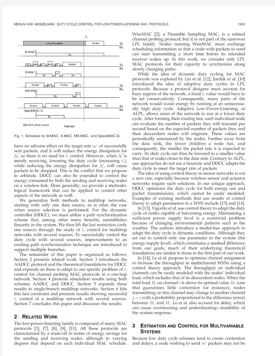
packet itself or an advertisement packet,in place of long preambles.The transmission schedules (hereafter “MAC schedule”)of some LPL MAC protocols are given in Fig.1.Previous work [9]has shown that,along a one-hop link,longer t i values favor receiving nodes,because longer t i values lower a node’s duty cycle while switching to Receive mode for the same period of time within the duty cycle.On the other hand,nodes that are mostly sending can greatly reduce their energy consumption if the t i value is low:They can stay in Sending mode for shorter periods of time.Consequently,there is a trade-off between the nodes at the two ends of a unidirectional wireless link.In addition,lower duty cycles often cause contention in areas of the network experiencing higher rates of packet transmissions.As Fig.1shows,only one data packet can be transmitted per cycle,which can cause a node to miss the target rate m ?of packet transmissions.In [10],Jurdak et al.convincingly argue that a fixed t i value does not fit WSN deployments where the node locations and traffic patterns are not uniform over the network.Because a fixed t i value is decided a priori,it would have to be set conservatively to accommodate areas in the network where traffic is expected to be heavy,thus forcing idle subregions to waste energy.In this paper,we propose two adaptive solutions to adjust the duty cycle.The first one is an intuitive linear increase/linear decrease scheme (AADCC).The second one (DDCC)borrows from control theory to dynamically adjust the duty cycle of the nodes based on a small set of parameters.We begin with one-hop networks.The goal of our methods is to minimize the energy consumed by the node with the lowest remaining energy (or the node which the application deems most important),referred to as node N ,while exchanging a target number of packets.If N is mostly sending,lowering t i (increasing the duty cycle)will .The authors are with the University of Rochester,Rochester,NY 14627.
E-mail:Christophe.Merlin@https://www.wendangku.net/doc/b511139770.html,,wheinzel@https://www.wendangku.net/doc/b511139770.html,.
Manuscript received 22Sept.2008;revised 26Jan.2010;accepted 25Apr.2010;published online 25June 2010.For information on obtaining reprints of this article,please send e-mail to:tmc@https://www.wendangku.net/doc/b511139770.html,,and reference IEEECS Log Number TMC-2008-09-0377.Digital Object Identifier no.10.1109/TMC.2010.116.
1.In his taxonomy of MAC protocols [4],Langendoen identifies Low-Power-Listening and Preamble Sampling protocols as two branches of random access MAC protocols,with the only difference that LPL MAC protocols need not know anything about their neighbors and their wake-up schedules.1536-1233/10/$26.00?2010IEEE Published by the IEEE CS,CASS,ComSoc,IES,&SPS
have no adverse effect on the target rate m?of successfully sent packets,and it will reduce the energy dissipation for N,so there is no need for t i control.However,when N is mostly receiving,lowering the duty cycle(increasing t i), while reducing the energy dissipation for N,will cause packets to be dropped.This is the conflict that we propose to arbitrate.DDCC can also be extended to control the energy consumed by both the sending and receiving nodes on a wireless link.More generally,we provide a methodo-logical framework that can be applied to control other aspects of the network as well.
We generalize both methods to multihop networks, starting with only one data source,as is often the case when source selection is performed.For the dynamic controller(DDCC),we must utilize a path synchronization scheme that,among other many benefits,reestablishes linearity in the system.We then lift the last restriction(only one source)through the study of t i control for multihop networks with several sources.To successfully control the duty cycle with several sources,improvements to an existing path synchronization technique are introduced to support multiple branches.
The remainder of this paper is organized as follows: Section2presents related work.Section3introduces the AADCC protocol and the theoretical foundations for DDCC and expands on these to adapt to our specific problem of t i control for channel probing MAC protocols in a one-hop network.Section4presents simulation results using both schemes AADCC and DDCC.Section5expands these results to single-branch multihop networks.Section6lifts this last constraint and presents results showing successful t i control of a multihop network with several sources. Section7concludes this paper and discusses the results. 2R ELATED W ORK
The low-power-listening family is composed of many MAC protocols[3],[7],[8],[9],[11].All these protocols are characterized by a trade-off in terms of energy savings for the sending and receiving nodes,although to varying degrees that depend on each individual MAC schedule.WiseMAC[2],a Preamble Sampling MAC,is a related channel probing protocol,but it is not part of the narrower LPL family.Nodes running WiseMAC must exchange scheduling information so that a node with packets to send can start transmitting a short time before its intended receiver wakes up.In this work,we consider only LPL MAC protocols for their capacity to synchronize along slowly changing paths.
While the idea of dynamic duty cycling for MAC protocols was explored by Lin et al.[12],Jurdak et al.[10] introduced the idea of adaptive duty cycles in LPL protocols.Because a protocol designer must account for busy regions of the network,a fixed t i value would have to be set conservatively.Consequently,many parts of the network would waste energy by running at an unnecessa-rily high duty cycle.Adaptive Low-Power-Listening,or ALPL,allows areas of the network to run at a lower duty cycle.After forming their routing tree,each individual node can evaluate the number of packets they will transmit per second based on the expected number of packets they and their descendant nodes will originate.These values are periodically announced by the nodes.Further away from the data sink,the fewer children a node has,and consequently,the smaller the packet rate it is expected to carry.Its duty cycle can thus be lowered to a smaller value than that of nodes closer to the data sink.Contrary to ALPL, our approaches do not use a heuristic and DDCC adapts the duty cycle to meet the target rate of packets.
The idea of using control theory in sensor networks is not a new one,especially because wireless sensor and actuator networks require such solutions.In our unique approach, DDCC optimizes the duty cycle for both energy use and packet transmissions,which cannot be easily modeled. Examples of existing methods that use results of control theory to adapt parameters in a WSN include[13]and[14].
In[13],Vigorito et https://www.wendangku.net/doc/b511139770.html,e control theory to adapt the duty cycle of nodes capable of harvesting energy.Maintaining a sufficient power supply level is a nontrivial problem because of changing environmental patterns such as the weather.The authors introduce a model-free approach to adapt the duty cycle in dynamic conditions.Although they set out to control only one parameter in the system(the energy supply level),which constitutes a marked difference from our goals,much of their underlying theoretical foundations are similar to those in the first part of our work.
In[14],Le et al.propose to optimize channel assignment to increase the throughput in multichannel WSNs using a control theory approach.The throughput on individual channels can be easily modeled with the nodes’individual load,which includes that of its descendant nodes.When the total load M i on channel i is above its optimal value M r(one that guarantees little contention for instance),nodes transmitting on this channel may change to another channel j?i with a probability proportional to the difference(error) between M r and M i.Le et al.also account for delay,which can cause overshooting and undershooting—instability of the system response.
3E STIMATION AND C ONTROL FOR M ULTIVARIABLE S YSTEMS
Because low duty cycle schemes tend to create contention and delays,a node wishing to send m?packets may not be
Fig.1.Schedule for B-MAC,X-MAC,MX-MAC,and SpeckMAC-D.
able to do so in a timely manner.Let us consider a one-hop network with various flows among neighbors.Node A wants to send m?packets to node B in a certain time period T, where node B is designated as node N,a critical node for the application,or one with very low remaining energy. Unfortunately,the medium is sometimes occupied by other transmissions.If node A only gets to send m 3.1Asymmetric Additive Duty Cycle Control The first proposed scheme is called asymmetric additive duty cycle control(AADCC).Protocol designers could easily find inspiration in the adaptive back-off scheme of the802.11MAC protocol.We chose to design our adaptive duty cycle control based on the number of consecutive packet transmissions.While802.11employs a multiplica-tive increase/linear decrease back-off,multiplicative in-crease turned out to be too disruptive in duty cycle control tests that we ran over the full range of t i values.Thus,we made our additive controller an asymmetric linear in-crease/linear decrease scheme.Whenever five consecutive packets are successfully sent to the destination,t i is increased by100ms,or t ieekt1TTT?t iek TTt0:1.Each failed packet is followed by a decrease of250ms in t i,or t ieekt1TTT?t iek TTà0:25.While this simple additive controller can produce better results than a static t i value, it cannot provide the optimal solution,as it does not consider energy dissipation or even try to approach a target m?.Therefore,our second scheme,DDCC,is based on control theory to optimize t i such that the target number of packets is sent while reducing energy dissipation. 3.2Background for Dynamic Control Here,we provide the mathematical background for our dynamic controller. 3.2.1Generalities We start by assuming that the system,we wish to represent and control,is mostly linear.For instance,the relationship between energy consumption and t i is linear,as energy consumption grows linearly with the number of probes done per second.Likewise,the number of packets received is mostly linearly related to energy consumption. Fig.2illustrates the system at hand.The network is represented by a“plant”that reacts to an input uetTby producing an output yetT,which it tries to match to a reference retT.A controller modifies uetTso as to obtain the desired output y?etT?retT.In order to do so,the process under control can be defined by its state xetT.A deterministic noisy linear process can be represented in its discrete form as follows: xett1T?AxetTtBuetTtCwetTtwett1T;e1Twhere xett1Tdesignates the value of the system state at timeekt1TT and w is the noise.T represents the period between reevaluations of the control uetT. For controlling t ietT,we can set yetTto metT(the number of packets that are successfully sent at time t)and uetTto the t ietTvalue at time t.The objective value y?ett1Tbecomes m?ett1T,the desired number of packets to be transmitted at time tt1. Because the fundamental characteristics of the system(A, B,and C)and its state xetTcannot be a priori known,the system’s output must be estimated using an internal parameter and a history of p values of f xetTg(or f yetTg) and f uetTg values stored in . 3.3The Dynamic Regulator In this first part of our work,we would like to control t i to send the target number of packets m?.We introduce a SISO (single variable)estimator and controller. 3.3.1Stochastic SISO Estimator and Controller We begin with the formulation of our goal,i.e.,the minimization of the expected error between the desired output at time tt1,y?ett1Tand the actual output at time tt1,yett1T,which is mathematically represented by the following: J?E?eyett1Tày?ett1TT2 :e2TThis control problem is referred to as linear-quadratic:the system dynamics are linear(1),but the cost function to be minimized(2)is quadratic.Because the system response contains a random component(the exact wake-up timing between two neighbors),we study a system estimator and controller for the stochastic case. First,and as suggested in[15],we introduce the following notation for time delay: xetà1T?qà1xetT: We can write the system as yetT?ayetà1Ttbuetà1Ttcwetà1TtwetTe3T ,e1àaqà1TyetT?bqà1uetTte1tcqà1TwetT:e4TFrom[15],(3)can be put in the form Ceqà1Ty0ett1j tT? eqà1TyetTt eqà1TuetT;e5Twhere Ceqà1T?1àaqà1tqà1g0?1teg0àaTqà1; eqà1T?g0; eqà1T?b; 8 < : and y0represents the next value taken by y and g0is a constant. The control law is thus shown to be uetT? y?ett1Tteg0àaTy?etTàg0yetT b?0 : Fig.2.Representation of the system with input/output and its controller. Let g0àa?c, uetT?y?ett1Ttcy?etTàeatcTyetT b ;e6T which is also the control law used in[13].It follows easily that(6)minimizes the mean-square error function J. Next,we define the and vectors as etTT etT?^yett1T; where^yett1Tis the estimated system output at time tt1. As a starting point,we chose to keep only the previous values of the input and output,or p?1.From(6),we use the two vectors: etT? yetT uetT y?etT 2 4 3 5; etT? atc b àc 2 4 3 5: The estimator can be computed using the Normalized Least-Mean-Square Algorithm(NLMS)[15],[16]: ett1T? etTt etT etT etTT etTt! ?yett1Tà etTT etT ;e7T where etTis a scalar,and!should be chosen to avoid a division by zero when etTT etTis null.With our notations, etTis thus the values of the output yetT?metT,the command uetT?t ietTand the target y?etT?m?etT.The tuple f a;b;c g is estimated using(7). New t i values are computed periodically.During each round(of duration T),the number of packets successfully transmitted since the last t i update(i.e.,metT)is recorded. 3.3.2Application to Our Estimator The system control can be approached by estimating the system first,and using the system model to find the input value that minimizes the predicted output. Preliminary results show that,while the estimator is able to correctly predict the system output,the control law tends to decrease the value of t ietTwhen m in fact to be expected as the system should decrease its duty cycle to increase the number of packet transmissions. Unfortunately,since J carries no consideration for energy use,t i never increases,even after the number of packets to be sent has reached the target(m?m?).The reason is that the error between^m and m?is zero,which does not modify the value of the controlled input uetT?t ietT.Fig.3a illustrates this problem.At t?500s,the packet rate increases to one packet per second,causing t i to decrease due to packet losses.However,a few seconds later,the packet rate decreases to its original value of0.5packet per second,yet t i does not increase again. Fig.3b shows the packet loss in this scenario,where the number of dropped packets is13for the dynamic controller (DDCC),and8for the additive controller(AADCC).The number of dropped packets is higher for the dynamic controller because it did not increase its duty cycle as aggressively.However,it preserved more of the nodes’energy(around10percent,not shown).Compared to a case without any duty cycle control(not shown),the number of dropped packets is reduced by over94percent by the duty cycle controller. Consideration must be given to the energy consumed , which is an incentive to lower the duty cycle.We note ?ett1Tas a target energy consumption at tt1. In this,now,multivariable case,we decided to estimate both the number of packets sent and the consumed energy separately.For m and ,the and vectors are m k ?m k...m kàp t ik...t ikàp m?k...m?kàp ??T ; m k ?a m0...a m pà1b m0...b m pà1c m0...c m pà1 ??T ; k ? k... kàp t ik...t ikàp m?k...m?kàp ??T ; k ?a 0...a pà1b 0...b pà1c 0...c pà1 ??T ; where a;b;c2I R are the estimator coefficients.We chose p>%3,a value that allows the estimate for and m to be accurate,while being still manageable in limited memory space. Fig.3.(a)Evolution of t ietTas the packet rate increases and then decreases when only packet loss is considered.(b)Packet loss in the same scenario. 3.3.3Cost Minimization As per Section 3.3.2,the controller should minimize a cost function with a packet loss and an energy component.We tried to combine the two costs in various ways,including taking the maximum,the sum,and the weighted sum of the costs.The latter offered the swiftest and most stable response from the network.Thus,the controller attempts to minimize the following cost function J : J ?em ?tà^m k t1T2tK e ?tà^ k t1T2;e8T where ^m k t1? mT k m k ; ^ k t1? T k k ; &m ?tand ?tdesignate the target values of m and at time ek t1TT .K is a weight given to the energy component of the cost function in order to indicate a preference to save energy (large K )or to strictly meet the number of packets to be sent (small K );for instance,K can be chosen in [2], [20].The control law finds the value of t i that minimizes J . Taking the derivative of J at time k T (we omit the k index notation for clarity),we obtain (6)for our application t i ? m p em ?tàP u i ?p m i m i TtK p e ?tàP v i ?p i i T e m p T2 tK e p T2; where the i -index value on i and i are the i th value of these vectors,and u and v are the number of elements in m k and k (u ?2p and v ?3p ).In order to smooth the response of the system,we adopt a conservative update policy "u for the duty cycle with the following set of rules: "t ik t1?"t ik t et i à"t ik T; "u k t1?f á ?"t ik t1 ;&e9T where "t i is the smoothed t i and f á ?x ? ;if x < ;á;if x >á; x;otherwise : 8 <: and áare the minimum and maximum values that t i can ever take,and can be set to 0.1and 5s as reasonable values. 2I R is the slope of the update of t i and helps stabilize the system response,which would otherwise be unstable because of steep variations of the reference r et T(the desired number of packets for instance)and delays in the feedback. A large (i.e.,close to 1)aggressively updates t i and incurs oscillations before reaching a determined value.On the other hand,if is close to 0,no oscillations can be discerned but t i is slow to reach its eventual value.Poor choices of may cause energy waste or packet loss.The command used to control the duty cycle is in fact "u as a smoothed output is critical to a physical network. 3.4Evaluating the Target Energy 3.4.1The Evaluation of and ? In some cases,the system designer may want to minimize the consumed energy and choose ??0.The risk incurred by this approach is that the duty cycle will tend to be lowered,even below a reasonable value—one that strikes a balance between the number of lost packets and energy consumption.This could be desirable when designing a system that needs to respond faster to lower energy consumption,and that can tolerate repeated packet losses.In other systems,an acceptable energy consumption value has to be evaluated so that t i et Tdoes not consistently increase past a reasonable value.This target energy has critical importance as the system will have a tendency to stabilize around the value of t i that yields this energy consumption,provided all packets are correctly sent.The control problem thus becomes a linear quadratic tracking (“LQ tracking”)problem where the output of the network must match the energy (and packet delivery)reference.We chose to evaluate the target energy as the sum of several basic operations (channel probe,packet reception,etc.)for which we precisely measured the energy consump-tion via a data acquisition board on the Tmote Sky platform.We evaluate the target energy as the minimal energy that can be expended during a round of T seconds: ??max e0;m ?E ?E Rx tE PD et T àm ?E ?t Rx TT;e10Twhere E ?E Rx is the expected energy spent to receive a packet,E PD is the energy consumed by the radio for one second of power down mode,and t T is the duration of a feedback round T .The target energy ?assumes that each packet is sent every t i s ,and that no energy is wasted on probing a clear channel.It contains no information about other transmissions in the neighborhood as packet loss is taken into account in the first element of J .3.4.2An Alternative Solution to Evaluating the Consumed Energy Because it maybe impractical to evaluate the energy consumption components and ?,an alternative solution is to use the linear increase of AADCC.This reduces the complexity of the system to only one component m .The relative simplicity of linear increase is offset by the slower nature of the response to increase t i when the data load diminishes.For DDCC in general,we prefer evaluating the energy,but we show in our later results that such a method where energy is not evaluated does provide satisfactory results.3.5Dynamic Duty Cycle Control Algorithm The controller,described in the previous theoretical foundations,is called Dynamic Duty Cycle Control (DDCC).Algorithm 3.1presents the pseudocode of DDCC.The initialization of the algorithm variables includes assigning a starting value to the and vectors. can take the initial values of m ?,t i ,and ?,while is initialized with values between à1and 1.For instance,an increase in t i translates into a decrease in m and of node N ,and thus the corresponding weights in are negative. Algorithm 3.1.DDCC pseudocode for p ?3 . In our implementation,we chose an initial ?0:01and then adjust to be 0.2after three iterations of the controller to prevent large oscillations during the first rounds of the estimators.Our network consists of 10nodes,all in range of one another (the medium can be occupied by only one node at a time).We evaluate the new command "u every T ? 5seconds:for instance,if a node sends packets at a rate of two packets per second,the controller will run every 2.5seconds.The feedback period T can be increased to reduce overhead,although a large value could cause the network adaptation to be sluggish—or worse,instable. 3.6Observations for an Implementation of the One-Hop Case For an implementation on real platforms in one-hop scenarios and for both controllers AADCC and DDCC, nodes need to periodically exchange information about their new t i values.For DDCC,nodes additionally need to exchange information about their remaining energy,using broadcast packets for instance,in order to determine the node N whose energy should be spared.If nodes A and B are possible choices for node N ,node A can elect to minimize the consumed energy at both nodes.DDCC works equally well by estimating the energy consumption at both A and B,although the t i value tends to be noisier. If a node is the receiving end of multiple links,it should adopt the smallest t i value t iL calculated by its descendants in order to receive all packets successfully.The amounts of energy wasted on the links using a lower duty cycle are negligible because the sending nodes will stop their packet transmissions after half t iL s on average—protocols like X-MAC and MX-MAC can interrupt their sending streams after receiving an ACK frame. Finally,if a node has multiple unicast destinations,a rare case in WSNs,which tend to have only one data sink,node A calculates the appropriate t i values for each link and sends them to the intended receivers individually.Support for multihop networks is introduced in Section 5.4S IMULATION R ESULTS FOR O NE -H OP N ETWORKS First,we observe the case when two nodes compete for the medium to send packets and only one node can modify its duty cycle.Then,we validate the duty cycle control when more than one node concurrently adjusts their t i values.4.1Method The radio behavior was modeled not only after the CC2420data sheet,but more importantly after the energy use of the whole Tmote Sky platform running a TinyOS implementa-tion.Although we present simulation results,our model closely resembles a real-life deployment,typically within three percent of the measured energy consumption [9].Here,the term simulation designates an accurate reconstruction of the reality.The choice of running simulations rather than an actual implementation was prompted by the difficulty in measuring energy consumption in real implementations:for LPL schemes,energy use does not degrade rapidly enough to collect usable and accurate data.An additional reason came with the objective of this work,which was to set the theoretical background for,and prove the feasibility of,t i control.In our discussion of the results,we often refer to a “fixed duty cycle”case,which is the scenario when the t i value is set at the beginning of the simulation and never changes (no duty cycle control).We ran such scenario simulations,but did not include their results on our graphs for clarity and space considerations.4.2Lowering the Duty Cycle to Save Energy:Demonstration of Principle Without the ability to adapt t i ,nodes running a LPL MAC protocol would force designers to select a high duty cycle at deployment to ease contention in busy areas of the network.Consequently,we start with a t i value of 300ms,with two nodes sending packets at an initial rate of 0.5packet per second.Fig.4presents the evolution of t i as well as the scenario of the simulation.Because a lower duty cycle can comfortably accommodate concurrent packet rates of 0:5pkt :s à1,the value of t i increases from 300to around 900ms in 1,500s (25min)for both AADCC and DDCC controllers.At this Fig.4.Evolution of t i et Tas the packet rate varies. point,the other packet source is turned off,and the packet rate of the remaining node is increased to1pkt:sà1.The t i value remains around950ms,as this t i value translates into an energy consumption within close range of the target energy.After2,000s,the packet rate is halved to0:5pkt:sà1. This allows the duty cycle to decrease further,as t i goes from 950to1.2s.Only10packets were lost during this scenario,in spite of the vigorous increase in t i. When compared to AADCC,DDCC helped reduce energy consumption by close to three percent(not shown) at the end of the simulation(close to a19percent reduction when compared to the fixed duty cycle case).As the later part of this scenario continues(after2,000s),this number will increase. 4.3Effect of the Feedback Period T We ran the same scenario as before for DDCC only,and changed the number of packets that are scheduled to be sent between evaluations of t i to test their impact.We doubled and quadrupled the value of T,or evaluated t i every10and 20packets.Fig.5shows that there is little difference between periods of5and10packets.For10packets,the evolution of t i appears to be smoother because of fewer updates.There is a greater difference between the t i values calculated between transmissions of5and20packets:the error on the estimation of the target energy is multiplied fourfold, and causes the duty cycle to often be higher than needed. 4.4Packet Loss Minimization We now study the other variable of interest by observing the number of lost packets.This example differs from the previous one in the initial value of t i(now1.5s)and in the number of neighbors transmitting over time.While it is unlikely that a protocol designer would choose such a high value for t i in a“fixed”case(no available control at all),this part of our work shows the behavior of our control schemes when packet loss occurs. Fig.6a shows a decreasing t i as packets are dropped in both control cases.Repeated packet losses cause the duty cycle using DDCC to be increased by a greater amount.The t i value can be observed to increase slightly between two feedback periods T in the first25min of the runtime as the energy component(approximately equal to the packet loss component)pushes the energy consumption down and the t i value up.In the second part of the runtime,packet losses become more frequent as the t i value is unrealistically high compared to the packet rate,until it reaches less than1s. Design choices could allow for a more aggressive t i descent, which would prevent the“spikes”on t i,but this would slightly compromise the rate of the t i increase once the packet rate declines again.This illustrates once again the trade-off between energy consumption and packet loss that the dynamic scheme balances. DDCC was able to limit packet loss by88percent over the“fixed”(no-control)scenario.As the duty cycle is iteratively modified,the frequency of dropped packets https://www.wendangku.net/doc/b511139770.html,pared to AADCC,DDCC dropped44more packets(or146percent more)because it increased the duty cycle very aggressively.This is transposed on the energy side,shown in Fig.6b,where DDCC reduced energy consumption by9.2percent compared to AADCC.Over the Fig.5.Evolution of t ietTfor various values of T . Fig.6.Evolution of(a)t i and(b)energy over time under a changing scenario:from a low duty cycle to a higher one. noncontrolled case,the energy increased by seven percent (not shown).The reason is that,in general,the increase in packet deliveries is compensated by an increase in energy consumption.The fixed scheme consumes less energy because of two reasons:its duty cycle remains at a low value,and contention around the nodes forces both the sender and the receiver to sleep for longer periods of time instead of transmitting packets—a behavior that results in lower energy consumption. 4.5Multiple Controllers A legitimate concern of t i control deals with the imple-mentation of several nodes adapting their duty cycles at the same time,particularly for a dynamic controller:The modifications of one should not destabilize the others. Fig.7shows that this is not the case as two sending nodes(nodes1and2)correctly adapt their duty cycles to conditions in the local area.The“cumulative t i”is the sum of the t i values of the sending nodes and can be seen as a measure of the busyness of a local area. 5t i C ONTROL FOR M ULTIHOP N ETWORKS The previous section validates the principle behind t i control for one-hop networks.In this section,we expand this work to single-branch multihop networks:Only one data source sends packets to one data sink several hops away. In this part of the work,the source(node0)intends to send m?packets to the destination(node n).Each packet travels along the same slowly changing path(i.e.,constant for a long period of time,corresponding to our simulation time for instance)over h?n hops.Each node keeps a queue of a maximum of100packets. 5.1Challenges Introduced by Multihop Control Although it is fairly inconsequential for the additive controller AADCC,the introduction of several hops along a source-destination path complicates key aspects of dynamic t i control(DDCC):The delay between the beginning of a transmission at the source and its reception at the destination greatly increases.This delay is exacer-bated by the nature of LPL MAC protocols because they rely on duty cycling.One consequence for dynamic t i control is that instability increases,although it can be compensated by a smaller updating slope of the command uetT—we lower it to0.1or less. Most importantly,the larger number of hops on the path induces nonlinearities in the system.Before a packet can be transmitted,a node must wait for the packet’s next hop to wake up.At every link along the path,the packet is held for a varying amount of time(although on average equal to t i=2s).Since the duty cycle is usually reevaluated every5to 10packets,the packet delay(and its corollary,the number of transmitted packets m)show wide variations from one feedback to the next,with little correlation to the t i value. In addition to this problem,two approaches to control the duty cycle can be considered:a per-link strategy and a per-path strategy.The former strategy offered the appeal of simply replicating the work done in Section3for every link along the path,and we tried it first.Investigative work rapidly showed that this approach could not be successful because queuing would happen at one point in the path, deceiving other nodes into increasing their t i because they correctly transmit m?packets.In general,this solution offered many untractable problems such as keeping a set of two values of t i at every node(one for the node itself,one for its next hop so that the first one could send to the second),coordinating together to avoid queuing,etc. Instead,the simple observation was made that since only one packet maybe transmitted by a node k every t i s, the nodes farther along the path(>k)would witness the same packet rate.Conversely,nodes placed before k would need to send at the same rate as k in order to maintain a constant queue at k.Therefore,we opted for a common duty cycle among all the nodes of a path,avoiding queuing whenever possible. 5.2Node Synchronization Along a Path While per-path t i control eased many of the challenges we faced,nonlinearities remained the main obstacle to multi-hop duty cycle control.We solved this problem through node synchronization along a path. Certain LPL MAC protocols have the unique ability to synchronize without explicit notification(i.e.,without overhead)along a slowly changing one-branch path.These protocols are X-MAC[7],C-MAC[11],and MX-MAC[9].A node k following the schedule of either one of these protocols learns of its next-hop neighbor kt1’s wake-up time at the end of every unicast transmission,that is,when it receives an acknowledgment frame.It follows that a node k can decide to back-off by a small t S time so that it may wake up right before node kt1during the next cycle. Done at every node along a path of h hops,nodes are automatically synchronized after the h th packet has been successfully received.The details of node synchronization along a path are presented in[17]. Among other features,path synchronization allows urgent packets to be received and forwarded immediately (within the same t i period)without loss of synchrony. Broadcast packets do not break node synchronization either. More importantly,this technique reintroduces linearity in the system since nodes’wake-up times are separated by a constant amount of time t S s.Packet delays are equal to t Rxtt Stehà1Tet itt STfor regular packets,and ht Stt Rx Fig.7.Evolution of t i over time under a changing scenario for the two nodes with duty cycle control. for urgent ones,where t Rx is the time to receive a packet, approximately14ms on average for our packet size. Furthermore,path synchronization significantly reduces congestion by staggering node wake-up schedules.Because nodes wake up sequentially along the path,a packet transmission interferes with next-hop nodes only,and not previous-hop nodes.This greatly reduces the chance for collisions and back-off,which increases the accuracy of energy estimation at remote nodes. 5.3Impact on the Energy Component of J Because the wake-up schedules of nodes are staggered,the time to transmit a packet is predictable and almost constant (t Stt Rx),whatever the duration of t i.In addition,since there is only one data source per path,each relay node must receive and send the same number of packets.Therefore, the expected energy consumption is the same at every relay node along the path since both the energies to send and receive a packet are equal at every hop.This reinforces the decision to utilize path-long duty cycles. In the case of only one data source on the network, saving the energy of one particular node on a multihop path no longer applies since all relays are expected to consume the same energy.Consequently,to lower the energy consumption of every relay node,the number of probes must be lowered such that a node may only wake up to send or receive a packet.The data source or the data sink are notable exceptions,since the originator of the data does not receive packets.The data sink,which does not send packets,is generally a node with larger resources and is less likely to request its energy be spared.Unless specified otherwise,we discuss the more general results of the relay nodes,although similar techniques can be applied for the nodes at the extremities of the path,as is done in Section3. Along synchronized paths,the energy consumption is thus the lowest when t i is the highest but still allows the target number of packets m?to be received.Hence,the controller arbitrates the trade-off between lower energy consumption and the objective to send m?packets. 5.4Observations for an Implementation of the Multihop Case The control of the duty cycle using DDCC requires information now located more than one hop away.In this section,we discuss possible practical solutions for imple-menting multihop duty cycle control. 5.4.1Target Number of Packets In all cases,we set packets to the same high priority.This meant that for path synchronization,they were all treated as urgent,and could thus be delivered within the same t i period (ht Stt Rx s later).In this section,we discuss where to close the feedback loop,i.e.,which node should be the t i controller. Calculation at node0.The target number of packets m?now depends on the packet rate of the data source,located at the beginning of a multihop path.To calculate the new t i value every feedback period T,a node must know m?,as well as the actual number of packets m received by the destination n.Because all nodes are sharing the same t i value and because they are synchronized along the path,the number of packets sent by node0is equal to m,provided none of the packets are dropped for unforseen reasons(a bad radio state,localized noise spike,etc.). Calculation at node nà1.The previous technique does not guarantee proper delivery of m?packets at the destina-tion if some of the links along the path are faulty.Because node nà1receives an ACK frame every time the destination receives a packet,it can easily calculate m.For this reason, the next-to-last node can be chosen to perform t i control. This method maybe preferred by programmers who suspect that nodes may fail and that detection of such failures will be slow.However,there is an inherent trade-off between packet overhead to spread the new t i value and delivery reliability. 5.4.2New t i Value Dissemination After t iekt1Thas been calculated,the duty cycle control-ling node should communicate this new t i value to nodes on the transmission path using t iekTand by piggybacking the new value onto broadcast packets.For the family of LPL MAC protocols,bigger packets incur no significant extra energy consumption since the radio remains in sending mode for the same period of time(t i s)regardless of the packet length.Nodes can then start using the new calculated duty cycle.The cost of this operation is at most that of transmitting one broadcast packet every T s on the active data path.In order to be the most energy-efficient, this dissemination on the path should coincide with other network maintenance events.In WSNs,the directions of data packets is usually fixed over a small period of time (e.g.,$10T)and centripetal:packets tend to travel from peripheral nodes(with valuable information to report) toward the base station(with compute power).Conversely, broadcast packets,generally used for network maintenance such as route repair or service discovery,tend to flow in the opposite direction.Cross-layer optimizations could join other maintenance packets with our t i updates.It should be noted that the problem of t i dissemination is not unique to our proposed schemes,but common to the whole family of adaptive duty cycle protocols.In fact,this work benefits from path synchronization,a very energy-efficient techni-que for multihop unicast packet transmissions[9]. 5.4.3Energy Estimation The node running dynamic duty cycle control needs to estimate the energy consumed by other nodes without requiring them to report it.The reasons to proceed in this way are threefold: .Good modeling:we were able to closely measure and model LPL MAC protocol energy consumption. Our model was found to be typically within three percent of testbed measurements. .Energy evaluation in isolation:nodes would also have to evaluate the energy consumed only by their own LPL MAC protocol because they maybe running other processes(packet processing,sensing activity,and packet aggregation)that draw energy but are not relevant to the MAC links. .Poor measuring tools:platforms like the Tmote Sky can only measure their battery voltage,which can be mapped to remaining energy but does not yield a sufficient precision when energy consumption is small(as is typically the case in LPL MAC protocols). Errors made in the evaluation of the energy consumption are modeled in the noise component of the system. 5.5Simulation Results We used Matlab to simulate these different strategies for a four-hop network with only one source.The control of the duty cycle was strikingly similar,whether t i was calculated at node0or node nà1.However,our simulation did not model unforseen congestion at nodes>1(caused by other transmissions in the vicinity of a node for instance),thus allowing the controller at node0to perform equally well. In this section,we present results obtained when node nà1is the controller,as in Section6. We first present results that were obtained through the direct evaluation of the consumed energy.Fig.8a shows the evolution of the duty cycle of the nodes when the packet rate of the source changes over time.When the packet rate of source node0doubles after400s,it fails to send m?packets per T period.Both controllers are successful in bringing the duty cycle to a value that allows the target number of packets to be reached(0.9s for AADCC and1s for DDCC).Because DDCC has an energy component in its command computation,it is sometimes too eager to increase t i.We see an example of this here.When the packet rate returns to0:5pkt:sà1,the duty cycle decreases again,providing t i around1.2s.Because we opted for a small update rate ?0:1,the dynamically controlled t i value increases slowly. Fig.8b shows that t i control reduces the number of packets failing to be https://www.wendangku.net/doc/b511139770.html,pared to the case without a controller,this reduction reaches a factor of four (not shown).The packets transmitted by node0to node1 are delivered to the destination within the same cycle.For the fixed duty cycle case,however,packets must be queued between400and1,250s.While queued packets can be eventually sent to the destination after the packet rate decreases,stale information is of little use to the application. Compared to AADCC,the number of dropped packets is similar for DDCC(13versus17,or40percent)with no queuing happening in either case. The energy consumption of DDCC is comparable, although lower than that of AADCC by two percent(not shown).Compared to the noncontrolled case,the improve-ment in packet delivery is obtained by a relative increase in energy consumption of10percent at relay nodes after2,000s, although the eventual energy consumption at the relay node can be eased when the duty cycle returns to a low value. The second set of results is presented for the case when the energy consumption is not evaluated at the dynamic controller,and the command uetTis automatically increased by0.1s when5T have passed without packet loss(like the linear increase of AADCC). Fig.9a shows the correct reduction of t i to accommodate sending more packets with either controller.When the network is favorable to t i increase,the response of DDCC is much more sluggish than in the regular and the additive controller cases(in fact,the dynamic controller opposes artificial t i increases).However,this translates in fewer dropped packets(reduced by a factor of three in Fig.9b,or a factor of nine compared to the fixed duty cycle case),and in a lower energy consumption of three percent(higher by eight percent over the fixed duty cycle case). These results illustrate the trade-off existing between the two techniques for utilizing energy information in DDCC, described in Section 3.4.2:the speed of the response translates into different energy consumption and packet delivery ratios.The decision to implement one technique or the other depends on the application needs and constraints. 6t i C ONTROL FOR M ULTIHOP N ETWORKS WITH M ULTIPLE S OURCES While adaptation of our controllers to multihop networks has greatly expanded the applications of t i control,the limitation imposed by only one data source limits its use to networks performing source selection—target tracking or building monitoring networks are instances of these networks. In this section,we modify both t i control strategies to support multihop networks with multiple data sources: while the control engine remains the same as in the previous section,our synchronization technique was upgraded to support multiple sources converging into one branch. 6.1Path Synchronization with Multiple Sources The greatest challenge posed by the use of multiple sources does not directly fall onto the theory behind t i control,but https://www.wendangku.net/doc/b511139770.html,parison of(a)the evolution of t i and(b)the dropped packets for the dynamic controller and additive controller when the energy is evaluated. rather concerns how path synchronization can be main-tained when several sources are converging at one node. Let Fig.10represent a three-hop network with two sources (marked by?)sending packets to a common destination h?3.First,we define several terms used throughout in this section:a branch node refers to node k,as the location where several flows meet.Nodes from a packet source to the branch node form a branch.The nodes placed after the branch node are part of the root of the path. The current synchronization technique staggers node transmission schedules such that node kt1would wake-up t S s before the destination h,node k2t S s before h,etc.This forces both sources(more generally,all nodes kà1forming a link kà1!k)to wake up at almost the same time.While this maybe acceptable for low offered loads,it cannot accommodate high packet rates from both sources. 6.1.1Strategy The key idea to support the convergence of l flows to one node k consists in increasing the duty cycle of root nodes (!k).The t i value must be divided by l to accommodate fair access to node k by all sources kà1j.2 Upon receiving a new unicast packet,node k checks the ID of the previous hop and adds it to a neighbor table if not present already.If a new source is detected,node k modifies the received packet to include a MAC header containing the value l,the ID kt1of its next hop,and the ID of the new previous hop.The new t i value is calculated as t new i ?t new i;k ?t i;k l là1 : The packet is then broadcast to all immediate neighbors. Nodes k and kt1adopt the new duty cycle after forwarding the packet to their next-hop neighbor. The broadcast packet sent by node k need not specify who the new source node is:upon attempting to send a packet and finding a busy network,a node kà1j will back- off by t new i =l s until all schedules are staggered. 6.1.2Implementation in TinyOS We tested and implemented this synchronization technique in TinyOS[18]using the Tmote Sky platform[19].In order to gather results,we let Matlab collect information through a TinyOS gateway.One of the difficulties in showing path synchronization is the fact that probes are“silent”:nodes simply turn their radios in receive mode,and receive a packet or go back to sleep.Only packet transmissions can be reported and plotted.We show path synchronization through the timing of packet transmissions. Our test network consisted of four nodes,with two sources(00and01)sending to node1.The initial t i value was1:5s.The TinyOS code was successfully tested for more sources,but since they are harder to read,these results are not shown here. Fig.11illustrates the process of path synchronization with two sources sending data packets to a common destination every20and10s.The Y-axis indicates the ID of the transmitting node.During the first half-minute,the path is established through a simple route discovery protocol and only one source is turned on.It takes two packets to synchronize the first source,which can be observed by the narrowing of the transmission bars.After45s,the second source turns on and sends its packet.It is immediately followed by a broadcast packet(sent over the full duration of the t i interval).Immediately after,we can see that the schedules are staggered.After75s,node00sends a packet to node1,immediately followed(t i=2s later)by node01. Node1then forwards both packets successively. Fig.10.A multihop network with two sources kà10and kà11(?denotes a source). https://www.wendangku.net/doc/b511139770.html,parison of(a)the evolution of t i and(b)the dropped packets for the dynamic controller and additive controller cases when the energy is not evaluated as per Section3.4.2. 2.The notation kà1j,where0j node k on branch j. Fig.11b shows the packet delivery delay for both sources. Once the nodes are synchronized,the packet delay hovers around1s—except for each sources’fourth packet,because 01sends its data before1can forward the packet from00.The first packets for both sources experience almost the same long delay(greater than3s,although for different reasons:when source00sends its first packet,nodes are not yet synchro-nized,and packet delivery is delayed by long transmission times.We see this delay being reduced in the following packet because node1synchronizes with its next-hop neighbor.The first packet of the second source,however,is delayed by the transmission of the broadcast packet indicat-ing a new t i value.Since synchronization is already in place on the existing path,source01is synchronized with node1 with the first packet,which explains why the following packet(with ID2)from node01experiences low delay.6.2t i Control for Synchronized Paths with Multiple Sources Path synchronization with multiple sources causes the root of the path to use different t i values.This technique prevents DDCC from excessively increasing the duty cycle to support both sources with the same t https://www.wendangku.net/doc/b511139770.html,pared to that approach,path synchronization results in energy savings for the branches of the network since their t i value can be l times that of the root. Since the node controlling the duty cycle must learn about the target number of packets m?,it should be placed after the branch node.Thus,node nà1(the node immediately before the destination)is a good candidate to be the controller for a path with multiple branches.Upon starting and stopping its flow of packets,a source must notify the controller of the number of packets it needs to transmit every second.This value is piggybacked onto the unicast data packet and is read by the controller.After the new t i value has been computed, it is broadcast and flooded onto the path. While the synchronization technique has evolved to support multiple branches,the t i control engine has remained the same as that of Section5.This shows the robustness of the both control techniques designed for multihop cases. 6.3Simulation Results The tested network consists of two sources,as shown in Fig.12,sending packets over a four-hop path with initial t i of 1.25s.The controller is the node placed before the destination,and we compared both the AADCC and DDCC controllers.Both schemes benefit from path syn-chronization to guarantee fairness in the comparison. Fig.13a shows the evolution of the duty cycle for AADCC and DDCC.During the initial phase of the simulation,the network experiences difficulties delivering all its packets, and thus decreases t i.After400s,the second source is turned on,and the total packet rate is tripled.The branch synchronization process activates,which can be visualized by a division of t i by two.The duty cycle of the network with AADCC is still doubled because of the synchronization process taking place after a second source has been detected. The response from the DDCC is a controlled increase in the duty cycle to accommodate the new load.During this time, DDCC is a little too eager to increase the t i value,and occasionally exceeds a safe value(presumably around 500ms)that allows delivery of m?packets(the same is true of AADCC).At1,250s,the second source is turned back-off, and the duty cycle is reduced to save energy. Using DDCC,the network dropped the same number of packets as when using AADCC(it dropped fewer packets by a factor of six compared to the fixed duty cycle network): Fig.13b shows that packets are mostly lost in the moments after the second source is turned on.Immediately following its activation(after400s),a loss of five,then three packets push the t i value lower. Fig.11.(a)Successful path synchronization for two nodes sending data packets to a common destination.The packet rates are1=20and 1=10pkt:sà1. (b)The reduction in packet delay as the synchronization takes place. Fig.12.Topology of the tested network with two sources. Fig.13c shows the extra energy consumed at node2 (the node where the branches converge)when the duty cycle is increased.DDCC was able to balance dropped packets and energy consumption better than AADCC,as the energy consumption of the former is8.5percent lower (it is three percent higher compared to the fixed duty cycle case).There is a clear trade-off in using any sort of adaptive duty cycle controller between improvement in quality of service(through the increase in immediate delivery of packets)and energy consumption.However,it can be argued that although the energy expanded in the case of the fixed duty cycle scheme is lower(because of a lower duty cycle and contention forces nodes to sleep longer),it is done in vain since many of the packets fail to be delivered.When using a duty cycle controller,the proposed DDCC strikes a better balance between packet delivery and energy consumption than AADCC for this tested scenario. 7C ONCLUSIONS,D ISCUSSION,AND F UTURE W ORK 7.1Summary of Work Low-Power-Listening MAC protocols show great promise to increase WSN lifetime by reducing idle listening. However,such MAC protocols were typically reserved for networks with low packet rates so as to allow low duty cycles(and greater energy savings). In this paper,we introduce two adaptive duty cycle control schemes.The Asymmetric Additive Duty Cycle Control and the Dynamic Duty Cycle Control have differing performance, but both provide adaptive control to the duty cycle of LPL MAC protocols.Both schemes are capable of increasing the duty cycle when the number of packets to be transmitted cannot be accommodated,and they can both decrease the duty cycle to conserve energy.DDCC jointly optimizes the energy consumed at vulnerable nodes and the number of packets to be transmitted.This results in energy savings of2to 10percent compared to AADCC,and20percent compared to the fixed duty cycle case for single-hop networks.When they cannot lower energy(because they have to accommodate the transmission of more packets),both AADCC and DDCC succeed in drastically reducing the number of dropped packets compared to the fixed duty cycle case. We generalized these results to multihop networks with multiple sources.The key to successful t i control was using and improving a path synchronization technique that allowed linearity to be maintained in the system.In our experiment,we saw a reduction of dropped packets by a factor of six(compared to the fixed duty cycle case)when the offered load increases.The higher duty cycle caused only a limited increase in energy consumption. This work showed that t i control allows networks to respond to sudden bursts of packets as caused by the occurrence of an event in a monitoring network,making LPL MAC protocols suitable for a greater number of WSN applications.t i control allows the network to choose a very low duty cycle,thus saving considerable amounts of energy when the network load is low,while accommodating higher loads whenever needed. More importantly,the proposed DDCC method,which does not require knowledge of a system’s physical model, can also be applied to the control of many other parameters in a network. 7.2Discussion Although the balance of sent packets and energy consump-tion is closer to optimal when using DDCC(minimization of the error function),protocol designers may consider various aspects when deciding whether to implement additive https://www.wendangku.net/doc/b511139770.html,parison of(a)the evolution of t i,(b)the dropped packets, and(c)the energy consumed for the dynamic controller and additive controller cases for two sources in a multihop network. control or dynamic control.While DDCC generally provides t i values closer to the optimal values,its implementation requires selecting an update coefficient ,as well as determining if energy conservation is more important than packet delivery.These aspects guide the responsiveness of DDCC to packet loss or when the packet rate decreases.In the results presented in this work,DDCC proved to correctly handle packet losses and to respond swiftly by increasing the duty cycle(Figs.6,7,8,and13).When it comes to increasing t i when the packet rate decreases,DDCC is relatively sluggish.This is due to a small to prevent oscillations. On the other hand,AADCC brings t i down very quickly when a packet loss occurs,and it is incapable of adapting the amount of t i decrease or increase as it nears its target(unlike DDCC).However,AADCC is a simpler scheme that provides satisfactory results.The implementation of AADCC promises to be quicker,and to utilize much smaller computational resources.All these considerations may make one controller more attractive over the other. 7.3Future Work For our future work,we plan to adapt DDCC to real-life deployments.Other estimators maybe considered for our work:we could replace the NLMS algorithm by the Newton’s method of gradient descent.We plan to adapt our method of path synchronization and t i control to more particular networks such as those made of branches of branches. Finally,we plan to investigate the possible cross-layer interactions made possible by this work.In particular,we would like to explore the impact of duty cycle on route selection:the routing protocol may find alternate routes to nodes with very high duty cycles and little remaining energy. A CKNOWLEDGMENTS This work was supported in part by US National Science Foundation#CNS-0448046. R EFERENCES [1] A.El-Hoiydi,“Aloha with Preamble Sampling for Sporadic Traffic in Ad Hoc Wireless Sensor Networks,”Proc.IEEE Int’l Conf. Comm.(ICC’02),Apr.2002. [2] A.El-Hoiydi and J.D.Decotignie,“WiseMAC:An Ultra Low Power MAC Protocol for the Downlink of Infrastructure Wireless Sensor Networks,”Proc.Ninth IEEE https://www.wendangku.net/doc/b511139770.html,puters and Comm. (ISCC’04),June2004. [3]J.Polastre,J.Hill,and D.Culler,“Versatile Low Power Media Access for Wireless Sensor Networks,”Proc.Second ACM Conf. Embedded Networked Sensor Systems(SenSys’04),pp.95-107,Nov. 2004. [4]https://www.wendangku.net/doc/b511139770.html,ngendoen,“Medium Access Control in Wireless Sensor Networks,”Medium Access Control in Wireless Networks,vol.2, Nova Science Publishers,2007. [5]IEEE Std.802.15,IEEE Computer https://www.wendangku.net/doc/b511139770.html,N MAN Standards Committee,Wireless LAN Medium Access Control(MAC)and Physical Layer(PHY)Specifications for Low Rate Wireless Personal Area Networks(LR-WPANs),IEEE,2004. [6]Chipcon Products from Texas Instruments,“CC2420Data Sheet, 2.4GHz IEEE802.15.4/ZigBee-ready RF Transceiver,”http:// https://www.wendangku.net/doc/b511139770.html,/files/CC2420_Data_Sheet_1_3.pdf,2008. [7]M.Buettner,G.V.Yee,E.Anderson,and R.Han,“X-MAC:A Short Preamble MAC Protocol for Duty-Cycled Wireless Sensor Net-works,”Proc.Fourth ACM Conf.Embedded Networked Sensor Systems (SenSys’06),pp.307-320,Nov.2006. [8]K.-J.Wong and D.K.Arvind,“SpeckMAC:Low-Power Decen- tralised MAC Protocols for Low Data Rate Transmissions in Specknets,”Proc.Second IEEE Int’l Workshop Multi-Hop Ad Hoc Networks:From Theory to Reality(REALMAN’06),May2006.[9] C.J.Merlin and W.B.Heinzelman,“Node Synchronization for Minimizing Delay and Energy Consumption in Low-Power-Listening MAC Protocols,”Proc.IEEE Conf.Ad-Hoc and Sensor Systems(MASS),pp.265-274,https://www.wendangku.net/doc/b511139770.html,/ ~merlin/NodeSynchronization/NodeSyncURTR.pdf,Sept.2008. [10]R.Jurdak,P.Baldi,and C.V.Lopes,“Adaptive Low Power Listening for Wireless Sensor Networks,”IEEE Trans.Mobile Computing,vol.6,no.8,pp.988-1004,Aug.2007. [11]S.Liu,K.-W.Fan,and P.Sinha,“CMAC:An Energy Efficient MAC Layer Protocol Using Convergent Packet Forwarding for Wireless Sensor Networks,”Proc.Fourth IEEE Comm.Soc.Conf. Sensor and Ad Hoc Comm.and Networks(SECON’07),June2007. [12]P.Lin,C.Qiao,and X.Wang,“Medium Access Control With a Dynamic Duty Cycle For Sensor Networks,”Proc.IEEE Wireless Comm.and Networking Conf.(WCNC’04),vol.3,pp.1534-1539, Mar.2004. [13] C.M.Vigorito,D.Ganesan,and A.G.Barto,“Adaptive Control of Duty Cycling in Energy-Harvesting Wireless Sensor Networks,” Proc.Fourth IEEE Comm.Soc.Conf.Sensor and Ad Hoc Comm.and Networks(SECON’07),June2007. [14]H.K.Le,D.Henriksson,and T.Abdelzaher,“A Control Theory Approach to Throughput Optimization in Multi-Channel Collec-tion Sensor Networks,”Proc.Sixth Int’l https://www.wendangku.net/doc/b511139770.html,rmation Proces-sing in Sensor Networks(IPSN’07),Apr.2007. [15]G.C.Goodwin and K.S.Sin,Adaptive Filtering Prediction and Control.Prentice Hall,1984. [16]P.Kumar and P.Varaiya,Stochastic Systems.Prentice Hall,1986. [17] C.J.Merlin and W.B.Heinzelman,“Node Synchronization for Minimizing Delay and Energy Consumption in Low-Power-Listening MAC Protocols,”Proc.Fifth IEEE Conf.Mobile Ad-Hoc and Sensor Systems(MASS’08),Sept.2008. [18]J.Hill,R.Szewczyk,A.Woo,S.Hollar,D.Culler,and K.Pister, “System Architecture Directions for Network Sensors,”Proc. Ninth Int’l Conf.Architectural Support for Programming Languages and Operating Systems(ASPLOS),2000. [19]Moteiv Tmote Sky,https://www.wendangku.net/doc/b511139770.html,/tmote,2008. Christophe J.Merlin received the BS/MS double degree from the National Institute of Applied Sciences in Rennes,France,in2003, and the MS and PhD degrees in electrical engineering from the University of Rochester in 2006and2009,respectively.His interests are in wireless sensor networks,medium access con- trol,and data center energy efficiency.He is now a product marketing engineer with the Sentilla Corporation.He is a member of the IEEE. Wendi B.Heinzelman received the BS degree in electrical engineering from Cornell University in1995and the MS and PhD degrees in electrical engineering and computer science from the Massachusetts Institute of Technology in1997and2000,respectively.She is an associate professor in the Department of Elec- trical and Computer Engineering at the Univer- sity of Rochester,and she holds a secondary appointment as an associate professor in the Department of Computer Science.She also currently serves as dean of graduate studies for arts,sciences,and engineering at the University of Rochester.Her current research interests lie in the areas of wireless communications and networking,mobile computing,and multimedia communication.She received the US National Science Foundation CAREER award in2005for her research on cross-layer architectures for wireless sensor networks,and she received the ONR Young Investi-gator award in2005for her work on balancing resource utilization in wireless sensor networks.She is an associate editor for the IEEE Transactions on Mobile Computing,the ACM Transactions on Sensor Networks,and the Elsevier Ad Hoc Networks Journal.She is a senior member of the IEEE and the ACM,and she is cofounder of the N2Women(Networking Networking Women)group. .For more information on this or any other computing topic, please visit our Digital Library at https://www.wendangku.net/doc/b511139770.html,/publications/dlib. 家装用尺寸一览表 Revised by Hanlin on 10 January 2021 家装用尺寸一览表 ▌标准入户门洞0.9m*2m, ▌房间门洞0.9m*2m, ▌厨房门洞0.8m*2m, ▌卫生间门洞0.7m*2m ▌客厅:长沙发:240*90*75cm长方形茶几:130*70*45cm电视柜:200*50*180cm电视离沙发:3m电视高度与电视柜高差:40到120cm走道宽度:100至120cm ▌厨房:橱柜操作台:台面高80cm左右面积90*46(最小20最大60)cm吊柜:离台面60cm左右高度在145cm到150cm餐桌:餐桌高:750—790mm。餐椅高;450—500mm。圆桌直径:二人500mm.二人800mm,四人900mm,五人1100mm,六人1100-1250mm,八人1300mm,十人l500mm,十二人1800mm。方餐桌尺寸:二人700×850(mm),四人1350×850(mm),八人2250×850(mm) ▌卫生间:浴缸长度:一般有三种1220、1520、1680mm;宽:720mm,高:450mm。坐便:750×350(mm)。冲洗器:690×350(mm)。盟洗盆:550×410(mm)。淋浴器高:2100mm。化妆台:长:1350mm;宽450mm。 ▌卧室:标准双人床尺寸:150*190、150*200厘米,被套的尺寸应配180*215和200*230之间的。加大双人床尺寸:180*200厘米,被套一般为200*230或220*240。床头柜宽:400毫米-600毫米,深:350毫米-450毫米高:500毫米-700毫米。衣柜:柜门尺寸,单 家具设计的基本尺寸(单位:cm) 衣橱:深度:一般60~65;推拉门:70,衣橱门宽度:40~65 推拉门:75~150,高度:190~240 矮柜:深度:35~45,柜门宽度:30-60 电视柜:深度:45-60,高度:60-70 单人床:宽度:90,105,120;长度:180,186,200,210 双人床:宽度:135,150,180;长度180,186,200,210 圆床:直径:186,212.5,242.4(常用) 室内门:宽度:80-95,医院120;高度:190,200,210,220,240 厕所、厨房门:宽度:80,90;高度:190,200,210 窗帘盒:高度:12-18;深度:单层布12;双层布16-18(实际尺寸) 沙发:单人式:长度:80-95,深度:85-90;坐垫高:35-42;背高:70-90 双人式:长度:126-150;深度:80-90 三人式:长度:175-196;深度:80-90 四人式:长度:232-252;深度80-90 茶几:小型,长方形:长度60-75,宽度45-60,高度38-50(38最佳) 中型,长方形:长度120-135;宽度38-50或者60-75 正方形:长度75-90,高度43-50 大型,长方形:长度150-180,宽度60-80,高度33-42(33最佳) 圆形:直径75,90,105,120;高度:33-42 方形:宽度90,105,120,135,150;高度33-42 书桌:固定式:深度45-70(60最佳),高度75 活动式:深度65-80,高度75-78 书桌下缘离地至少58;长度:最少90(150-180最佳) 餐桌:高度75-78(一般),西式高度68-72,一般方桌宽度120,90,75;长方桌宽度80,90,105,120;长度150,165,180,210,240 圆桌:直径90,120,135,150,180 书架:深度25-40(每一格),长度:60-120;下大上小型下方深度35-45,高度80-90活动未及顶高柜:深度45,高度180-200 木隔间墙厚:6-10;内角材排距:长度(45-60)*90 家具设计的基本尺寸(单位:厘米) 衣橱:深度:一般60~65;推拉门:70,衣橱门宽度:40~65 推拉门:75~150,高度:190~240 矮柜:?深度:35~45,柜门宽度:30-60 电视柜:深度:45-60,高度:60-70 单人床:宽度:90,105,120;长度:180,186,200,210 双人床:宽度:135,150,180;长度180,186,200,210 圆床:?直径:186,,(常用) 室内门:宽度:80-95,医院120;高度:190,200,210,220,240 厕所、厨房门:宽度:80,90;高度:190,200,210 窗帘盒:高度:12-18;深度:单层布12;双层布16-18(实际尺寸) 沙发:单人式:长度:80-95,深度:85-90;坐垫高:35-42;背高:70-90双人式:长度:126-150;深度:80-90 三人式:长度:175-196;深度:80-90 四人式:长度:232-252;深度80-90 茶几:小型,长方形:长度60-75,宽度45-60,高度38-50(38最佳) 中型,长方形:长度120-135;宽度38-50或者60-75 正方形:?长度75-90,高度43-50 大型,长方形:长度150-180,宽度60-80,高度33-42(33最佳) 圆形:直径75,90,105,120;高度:33-42 方形:宽度90,105,120,135,150;高度33-42 书桌:固定式:深度45-70(60最佳),高度75 活动式:深度65-80,高度75-78 书桌下缘离地至少58;长度:最少90(150-180最佳) 餐桌:高度75-78(一般),西式高度68-72,一般方桌宽度120,90,75; 长方桌宽度80,90,105,120;长度150,165,180,210,240 圆桌:直径90,120,135,150,180 书架:深度25-40(每一格),长度:60-120;下大上小型下方深度35-45,高度80-90 活动未及顶高柜:深度45,高度180-200 木隔间墙厚:6-10;内角材排距:长度(45-60)*90 桌类家具高度尺寸:700mm、720mm、740mm、760mm四个规格; 椅凳类家具的座面高度:400mm、420mm、440mm三个规格。 桌椅高度差应控制在280至320mm范围内。 提供全方位装修指南,装修设计知识、丰富设计案例! 家装各种最佳尺寸标准大全! 家装最实际的规格尺寸 标准红砖24*11.5*53; 标准入户门洞0.9米*2米, 房间门洞0.9米*2米, 厨房门洞0.8米*2米, 卫生间门洞0.7米*2米, 标准水泥50kg/袋。 厨房 1.吊柜和操作台之间的距离应该是多少? 60厘米。 从操作台到吊柜的底部,您应该确保这个距离。这样,在您可以方便烹饪的同时,还可以在吊柜里放一些小型家用电器。 2.在厨房两面相对的墙边都摆放各种家具和电器的情况下,中间应该留多大的距离才不会影响在厨房里做家务? 120厘米。 为了能方便地打开两边家具的柜门,就一定要保证至少留出这样的距离。 150厘米。 这样的距离就可以保证在两边柜门都打开的情况下,中间再站一个人。 3.要想舒服地坐在早餐桌的周围,凳子的合适高度应该是多少? 80厘米。 对于一张高110厘米的早餐桌来说,这是摆在它周围凳子的理想高度。因为在桌面和凳子之间还需要30厘米的空间来容下双腿。 4.吊柜应该装在多高的地方? 145至150厘米。 提供全方位装修指南,装修设计知识、丰富设计案例! 餐厅 1. 一个供六个人使用的餐桌有多大? 2. 120厘米。 这是对圆形餐桌的直径要求。 140*70厘米。 这是对长方形和椭圆形捉制的尺寸要求。 2.餐桌离墙应该有多远? 80厘米。 这个距离是包括把椅子拉出来,以及能使就餐的人方便活动的最小距离。 3.一张以对角线对墙的正方形桌子所占的面积要有多大? 180*180平方厘米。 这是一张边长90厘米,桌角离墙面最近距离为40厘米的正方形桌子所占的最小面积。 4.桌子的标准高度应是多少? 72厘米。 这是桌子的中等高度,而椅子是通常高度为45厘米。 5.一张供六个人使用的桌子摆起居室里要占多少面积? 300*300厘米。 需要为直径120厘米的桌子留出空地,同时还要为在桌子四周就餐的人留出活动空间。这个方案适合于那种大客厅,面积至少达到600*350厘米。 6.吊灯和桌面之间最合适的距离应该是多少? 70厘米。 这是能使桌面得到完整的、均匀照射的理想距离。 卫生间 1.卫生间里的用具要占多大地方? 马桶所占的一般面积: 37厘米×60厘米。 【精华】室内装修,必须预留的最佳尺寸标准大全 2014-08-29筑龙房地产筑龙房地产 阅读引语 强烈推荐大家存的一份装修预留尺寸标准!!非常实用!! 现在新房子的设计一般都会交给专门的设计师来做,但哪怕是专业设计师制作的设计图稿,没有实地接触的设计师可能还会存在一些设计尺寸上的死角。另 外,落实图稿的是施工队的工人,工人往往疏忽大意就会犯错。于是房子装修完了,总是小错误不断。因此小哥觉得大家有必要存一份尺寸标准,监工时要用起来 哦!且看且分享吧! PART1:【客 厅】 【面积:20平方米~40平方米】 客厅是居室的门面,可以说对家具尺寸的要求是最严格的,多大的沙发配多大的茶几,多远的距离适合摆放电视等等,别看都是一些小数字,却足以令你的客厅成为一个舒适协调的地方。 电视组合柜的最小尺寸? 【200×50×180厘米】 对于小户型的客厅,电视组合柜是非常实用的,这种类型的家具一般都是由大小不同的方格组成,上部比较适合摆放一些工艺品,柜体厚度至少要保持30厘米;而下部摆放电视的柜体厚度则至少要保持50厘米,同时在选购电视柜时也要考虑组合柜整体的高度和横宽与墙壁的面宽是否协调。 长沙发或是扶手沙发的椅背应该有多高? 【85至90厘米】 沙发是用来满足人们的放松与休息的需求,所以舒适度是最重要的,这样的高度可以将头完全放在*背上,让颈部得到充分放松。如果沙发的*背和扶手过低,建议增加一个*垫来获得舒适度,如果空间不是特别宽敞,沙发应该尽量靠墙摆放。 扶手沙发与电视机之间应该预留多大的距离? 【3米左右】 这里所指的是在一个29英寸的电视与扶手沙发或和长沙发之间最短的距离,此外,摆放电视机的柜面高度应该在40厘米到120厘米之间,这样才能让看者非常舒适。 与容纳三个人的沙发搭配,多大的茶几合适呢? 【120×70×45厘米或100×100×45厘米】 在沙发的体积很大或是两个长沙发摆在一起的情况下,矮茶几就是很好的选择,茶几的高度最好和沙发坐垫的位置持平。 目前市场上较为流行的是一种低矮的方几,材质多为实木或实木贴皮的,质感较好。 细节补充: 照明灯具距桌面的高度,白炽灯泡60瓦为100厘米,40瓦为65厘米,25瓦为50厘米,15瓦为30厘米;日光灯距桌面高度,40瓦为150厘米,30瓦为140厘米,20瓦为110厘米,8瓦为55厘米。 PART2:【餐 厅】 【面积:10平方米~20平方米】 用餐的地方是一家人团聚最多的地方,通常也是居室中较为拥挤的一个空间,因为有较多的餐椅需要放置,也是家人同时集中的地方,所以它的尺寸就更要精打细算才能使餐厅成为一个温馨的地方。 家具设计地基本尺寸(单位:) 衣橱:深度:一般;推拉门:,衣橱门宽度: 推拉门:,高度: 矮柜:深度:,柜门宽度: 电视柜:深度:,高度: 单人床:宽度:,,;长度:,,, 双人床:宽度:,,;长度,,, 圆床:直径:,,(常用) 室内门:宽度:,医院;高度:,,,, 厕所、厨房门:宽度:,;高度:,, 窗帘盒:高度:;深度:单层布;双层布(实际尺寸) 沙发:单人式:长度:,深度:;坐垫高:;背高: 双人式:长度:;深度: 三人式:长度:;深度: 四人式:长度:;深度 茶几:小型,长方形:长度,宽度,高度(最佳) 中型,长方形:长度;宽度或者 正方形:长度,高度 大型,长方形:长度,宽度,高度(最佳) 圆形:直径,,,;高度: 方形:宽度,,,,;高度 书桌:固定式:深度(最佳),高度 活动式:深度,高度 书桌下缘离地至少;长度:最少(最佳) 餐桌:高度(一般),西式高度,一般方桌宽度,,;长方桌宽度,,,;长度,,,,圆桌:直径,,,, 书架:深度(每一格),长度:;下大上小型下方深度,高度 活动未及顶高柜:深度,高度 木隔间墙厚:;内角材排距:长度()* 室内常用尺寸 、墙面尺寸 ()踢脚板高;—. ()墙裙高:—. ()挂镜线高:—(画中心距地面高度). .餐厅 () 餐桌高:—. () 餐椅高;—. () 圆桌直径:二人.二人,四人,五人,六人,八人,十人,十二人. () 方餐桌尺寸:二人×(),四人×(),八人×(), () 餐桌转盘直径;—. 餐桌间距:(其中座椅占)应大于. () 主通道宽:—. 内部工作道宽:—. () 酒吧台高:—,宽. () 酒吧凳高;一. 在客厅 .长沙发与摆在它面前地茶几之间地正确距离是多少? 厘米 在一个(**高厘米)地长沙发面前摆放一个(**高厘米)地长方形茶几是非常舒适地.两者之间地理想距离应该是能允许你一个人通过地同时又便于使用,也就是说不用站起来就可以方便地拿到桌上地杯子或者杂志. b5E2R。 .一个能摆放电视机地大型组合柜地最小尺寸应该是多少? **高厘米 这种类型地家具一般都是由大小不同地方格组成,高处部分比较适合用来摆放书籍,柜体厚度至少保持厘米;而低处用于摆放电视地柜体厚度至少保持厘米.同时组合柜整体地高度和横宽还要考虑与墙壁地面积相协调..如果摆放可容纳三、四个人地沙发,那么应该选择多大地茶几来搭配呢? **高厘米 在沙发地体积很大或是两个长沙发摆在一起地情况下,矮茶几就是很好地选择,高度最好和沙发坐垫地位置持平. .在扶手沙发和电视机之间应该预留多大地距离? 米 这里所指地是在一个英寸地电视与扶手沙发或长沙发之间最短地距离.此外,摆放电视机地柜面高度应该在厘米到厘米之间,这样才能使观众保持正确地坐姿. .摆在沙发边上茶几地理想尺寸是多少? 方形:**高厘米. 椭圆形:*高厘米. 放在沙发边上地咖啡桌应该有一个不是特别大地桌面,但要选那种较高地类型,这样即使坐着地时候也能方便舒适地取到桌上地东西. p1Ean。 .两个面对面放着地沙发和摆放在中间地茶几一共需要占据多大地空间? 两个双人沙发(规格 **高厘米)和茶几(规格**高厘米)之间应相距厘米. .长沙发或是扶手沙发地地靠背应该有多高? 装修常用家具尺寸 在工地 1、标准红砖23*11*6;标准入户门洞0.9米*2米,房间门洞0.9米*2米,厨房门洞0.8米*2米,卫生间门洞0.7米*2米,标准水泥50kg/袋。 在厨房 1.吊柜和操作台之间的距离应该是多少? 60厘米。 从操作台到吊柜的底部,您应该确保这个距离。这样,在您可以方便烹饪的同时,还可以在吊柜里放一些小型家用电器。 2.在厨房两面相对的墙边都摆放各种家具和电器的情况下,中间应该留多大的距离才不会影响在厨房里做家务? 120厘米。 为了能方便地打开两边家具的柜门,就一定要保证至少留出这样的距离。 150厘米。 这样的距离就可以保证在两边柜门都打开的情况下,中间再站一个人。 3.要想舒服地坐在早餐桌的周围,凳子的合适高度应该是多少? 80厘米。 对于一张高110厘米的早餐桌来说,这是摆在它周围凳子的理想高度。因为在桌面和凳子之间还需要30厘米的空间来容下双腿。 4.吊柜应该装在多高的地方? 145至150厘米。 这个高度可以使您不用垫起脚尖就能打开吊柜的门。 在餐厅 1.一个供六个人使用的餐桌有多大? 120厘米。 这是对圆形餐桌的直径要求。 140*70厘米。 这是对长方形和椭圆形捉制的尺寸要求。 2.餐桌离墙应该有多远? 80厘米。 这个距离是包括把椅子拉出来,以及能使就餐的人方便活动的最小距离。 3.一张以对角线对墙的正方形桌子所占的面积要有多大? 180*180平方厘米 这是一张边长90厘米,桌角离墙面最近距离为40厘米的正方形桌子所占的最小面积。 4.桌子的标准高度应是多少? 72厘米。 这是桌子的中等高度,而椅子是通常高度为45厘米。 5.一张供六个人使用的桌子摆起居室里要占多少面积? 300*300厘米。 需要为直径120厘米的桌子留出空地,同时还要为在桌子四周就餐的人留出活动空间。这个方案适合于那种大客厅,面积至少达到600*350厘米。 6.吊灯和桌面之间最合适的距离应该是多少? 70厘米。 这是能使桌面得到完整的、均匀照射的理想距离。 在卫生间 1.卫生间里的用具要占多大地方? 马桶所占的一般面积:37厘米×60厘米 悬挂式或圆柱式盥洗池可能占用的面积:70厘米×60厘米 正方形淋浴间的面积:80厘米×80厘米 浴缸的标准面积:160厘米×70厘米 2.浴缸与对面的墙之间的距离要有多远? 100厘米。想要在周围活动的话这是个合理的距离。即使浴室很窄,也要在安装浴缸时留出走动的空间。总之浴缸和其他墙面或物品之间至少要有60厘米的距离。 干货│家装尺寸数据大全,大家快掏 出小本本记好了! 一、那些在工地的数据 (3) 二、那些在客厅涉及的家装数据 (4) 三、那些在厨房涉及到的家装数据 (8) 四、那些在餐厅涉及到的家装数据 (9) 五、那些在卫生间涉及到的家装数据 (11) 装修从来不是一件一蹴而就的事 它是一项关乎未来几十年生活质量的细活儿 可以精确到一丝一毫 因此了解一些家具尺寸的数据是非常必要的常识 为了有效避免以下惨烈装修车祸现场 比如心爱的沙发多出一块经常绊倒人 又比如一眼看中的床卧室竟然放不下······ 下面各位装修的宝宝赶紧来围观一起涨姿势 一、那些在工地的数据 1、标准红砖23*11*6; 2、标准入户门洞0.9米*2米, 3、房间门洞0.9米*2米, 4、厨房门洞0.8米*2米, 5、卫生间门洞0.7米*2米, 6、标准水泥50kg/袋。 二、那些在客厅涉及的家装数据 1.长沙发与摆放在它面前的茶几之间的正确距离是多少? 30厘米在一个(240*90*75高厘米)的长沙发面前摆放一个(130*70*45高厘米)的长方形茶几是非常舒适的。两者之间的理想距离应该是能允许你一个人通过的同时又便于使用,也就是说不用站起来就可以方便地拿到桌上的杯子或者杂志。 2.一个能摆放电视机的大型组合柜的最小尺寸应该是多少? 200*50*180厘米这种类型的家具一般都是由大小不同的方格组成,高处部分比较适合用来摆放书籍,柜体厚度至少保持30厘米;而低处用于摆放电视的柜体 厚度至少保持50厘米。同时组合柜整体的高度和横宽还要考虑与墙壁的面积相协调。 3.如果摆放可容纳三、四个人的沙发,那么应该选择多大的茶几来搭配呢?140*70*45高厘米。在沙发的体积很大或是两个长沙发摆在一起的情况下,矮茶几就是很好的选择,高度最好和沙发坐垫的位置持平。 4.在扶手沙发和电视机之间应该预留多大的距离? 3米。这里所指的是在一个25英寸的电视与扶手沙发或长沙发之间最短的距离。此外,摆放电视机的柜面高度应该在40厘米到120厘米之间,这样才能使观众保持正确的坐姿。 1.商品图片的尺寸:宽500*高500像素,大小在120KB以内,要求JPG或GIF格式,到发布宝贝页面上上传图片。最好大于312*310px 2.店标图片的尺寸:宽100*高100像素,大小在80K以内,支持JPG或GIF格式,动态或静态的图片均可。上传步骤:“管理我的店铺”-“基本设置”-“店标”-“浏览”-“确定” 3.宝贝描述图片的尺寸:没有特殊要求,可根据需要宽500*高500像素,大小在100K以内,这样图片的打开速度较快。要求JPG或GIF格式,静态或动态均可。将图片上传到电子相册,再复制到商品页面中去。 4.公告栏图片的尺寸:宽不超过480像素,长度不限制,大小在120KB以内GIF或JPG格式,动态或者静态均可。上传“管理我的店铺”-“基本设置”-“公告栏”-“确定”。 5.宝贝分类图片尺寸:宽不超过165,长度不限制,大小在50KB以内,要求GIF或JPG格式,动态或者静态均可,先将图片上传到电子相册得到一个缩短网址后进入“管理我的店铺”-“基本设置”-“宝贝分类” 6.旺旺头像图片尺寸:宽120*高120像素,大小在100KB以内,格式为JPG或GIF,动态或者静态均可。 7.论坛头像图片尺寸:最大为宽120*高120像素,大小在100KB以内,GIF或者JPG格式,动态或者静态图片均可。上传方法“我的淘宝”-“个人空间”-“修改资料”-“上传新头像”。 8.论坛签名档图片尺寸:宽468*高60像素,大小在100KB以内,JPG或者GIF格式,动态或者静态均可,上传“我的淘宝”-“个人空间 淘宝店铺装修最佳尺寸 普通店铺 1.店标 大小:100*100px <=80k 代码:无(图片做好后直接上传) 格式:jpg、gif 设置:管理我的店铺—基本设置—店标—浏览—选择本地做好店标文件 2. 店铺公告尺寸:320*400 3.宝贝分类尺寸:88*88和88*30(宝贝分类含3个) 4.店铺介绍尺寸:600*450 5.计数器尺寸:137*94 6.论坛签名尺寸:468*60 家里装修,最重要的是什么? 不是缤纷夺目的软装搭配设计,也不是酷炫十足的多功能变化装置,而是严格把控每一个细节尺寸,保证在装修完毕之后,根本的硬件设施合乎人体工程学的基本要求,让家里每个人住着舒适开心,这才是最重要的。这里,不仅整理出了完善的室内常见尺寸,更有一些独具风格的创意设计尺寸,让家装不再是难事。 室内常见家具的基本尺寸(单位:cm) 客厅篇 沙发: 单人式:长度:80-95,深度:85-90;坐垫高:35-42;背高:70-90 双人式:长度:126-150;深度:80-90 三人式:长度:175-196;深度:80-90 四人式:长度:232-252;深度80-90 茶几: 小型,长方形:长度60-75,宽度45-60,高度38-50(38最佳) 中型,长方形:长度120-135;宽度38-50或者60-75 正方形:长度75-90,高度43-50 大型,长方形:长度150-180,宽度60-80,高度33-42(33最佳) 圆形:直径75,90,105,120;高度:33-42 方形:宽度90,105,120,135,150;高度33-42 墙面尺寸: (1)踢脚板高:8—20 (2)墙裙高:80—150 (3)挂镜线高:160—180(画中心距地面高度) 厕所、厨房门:宽度:80,90;高度:190,200,210 窗帘盒:高度:12-18;深度:单层布12;双层布16-18(实际尺寸) 厨房餐厅篇 餐桌高:75—79 餐椅高:45—50 圆桌直径:二人50,二人80,四人90,五人110,六人110-125,八人130,十人l50,十二人180。 方餐桌尺寸:二人70×85,四人135×85,八人225×85 餐桌转盘直径:70—80 餐桌间距:(其中座椅占50)应大于50 主通道宽:120—130 内部工作道宽:60—90 酒吧台高:90—l05,宽50 酒吧凳高:60一75 卧室篇 衣橱:深度:一般60~65;推拉门:70,衣橱门宽度:40~65 推拉门:75~150,高度:190~240 矮柜:深度:35~45,柜门宽度:30-60 电视柜:深度:45-60,高度:60-70 单人床:宽度:90,105,120;长度:180,186,200,210 双人床:宽度:135,150,180;长度:180,186,200,210 圆床:直径:186,212.5,242.4(常用) 室内门:宽度:80-95,医院120;高度:190,200,210,220,240 书桌:固定式:深度45-70(60最佳),高度75 活动式:深度65-80,高度75-78 书桌下缘离地至少58;长度:最少90(150-180最佳) 圆桌:直径90,120,135,150,180 书架:深度25-40(每一格),长度:60-120;下大上小型下方深度35-45,高度80-90 木隔间墙厚:6-10;内角材排距:长度(45-60)*90 室内常用尺寸(单位:cm) 客厅篇 1.长沙发与茶几之间的距离 =30cm 在一个(240*90*75)的长沙发面前摆放一个(130*70*45)的长方形茶几是非常舒适的。是能允许一人通过的同时又便于使用的理想距离。 2.一个能摆放电视机的大型组合柜的最小尺寸=200*50*180 这种类型的家具一般都是由大小不同的方格组成,高处部分比较适合用来摆放书籍,柜体厚度至少保持30厘米;而低处用于摆放电视的柜体厚度至少保持50厘米。同时组合柜整体的高度和横宽还要考虑与墙壁的面积相协调。 3.如果摆放可容纳三、四个人的沙发,应该选择搭配的茶几大小=140*70*45 家具设计标准尺寸 家具设计的基本尺寸(单位:厘米 衣橱:深度:一般60~65;推拉门:70,衣橱门宽度:40~65 推拉门:75~150,高度:190~240 矮柜:深度:35~45,柜门宽度:30-60 电视柜:深度:45-60,高度:60-70 单人床:宽度:90,105,120;长度:180,186,200,210 双人床:宽度:135,150,180;长度180,186,200,210 圆床:直径:186,212.5,242.4(常用) 室内门:宽度:80-95,医院120;高度:190,200,210,220,240 厕所、厨房门:宽度:80,90;高度:190,200,210 窗帘盒:高度:12-18;深度:单层布12;双层布16-18(实际尺寸) 沙发:单人式:长度:80-95,深度:85-90;坐垫高:35-42;背高:70-90 双人式:长度:126-150;深度:80-90 三人式:长度:175-196;深度:80-90 四人式:长度:232-252;深度80-90 茶几:小型,长方形:长度60-75,宽度45-60,高度38-50(38最佳 中型,长方形:长度120-135;宽度38-50或者60-75 正方形:长度75-90,高度43-50 大型,长方形:长度150-180,宽度60-80,高度33-42(33最佳) 圆形:直径75,90,105,120;高度:33-42 方形:宽度90,105,120,135,150;高度33-42 书桌:固定式:深度45-70(60最佳),高度75 活动式:深度65-80,高度75-78 书桌下缘离地至少58;长度:最少90(150-180最佳) 餐桌:高度75-78(一般),西式高度68-72,一般方桌宽度120,90,75; 长方桌宽度80,90,105,120;长度150,165,180,210,240 圆桌:直径90,120,135,150,180 书架:深度25-40(每一格),长度:60-120;下大上小型下方深度35-45,高度80-90 活动未及顶高柜:深度45,高度180-200 木隔间墙厚:6-10;内角材排距:长度(45-60)*90 室内家具尺寸标准大全 ●电视柜尺寸: 电视组合柜最小尺寸:2000×500×1800毫米。 电视组合柜厚度:上部至少要300毫米,下部摆放电视的柜体至少要500毫米。电视柜面高度:在400—1200毫米,另一说在400-520毫米,又一说600—700毫米。电视柜:深度450—600毫米,高度600-700毫米。●沙发尺寸: 客厅尺寸篇(单位:mm) 01、沙发尺寸:一般深度800~900、坐位高350~420、背高700~900 单人式:长度:800-950,深度:850-900坐垫高:350-420;背高:70-90 双人式:长度:1260-1500;深度:800-900 三人式:长度:1750-1960;深度:800-900 四人式:长度:2320-2520;深度:800-900 02、茶几尺寸:茶几高度一般在330~420,但边角茶几有时稍高一些,为430~500 03、沙发和茶几之间的距离一般控制在300比较合适 04、一般电视机和沙发之间最短距离控制在3000 05、放置台式电视机的柜台高度,一般控制在400到1200之间 06、液晶电视机壁挂高度一般控制在电视机屏幕的中心点和观看电视时的视线平行,一般在1100,常规控制在1000-1500 餐厅尺寸篇(单位:mm) 一、餐桌尺寸 圆桌直径:二人500、三人800、四人900、五人1100、六人1200 (前几种规格圆桌人均占有弧长为600-800,以满负荷使用计算,一般固定其尺寸来使用) 八人1300-1400,十人1500-l600,十二人1800-2000 (此类推下去规格,人均占弧长控制在500-550,考虑非满负荷使用状况(餐桌转盘直径;700—800) 方桌尺寸: 此只探讨长条方桌,因正方方桌可通过长条方桌来推算其所需尺寸:一般短边控制在800-850, 长边则按人均占有计算:控制在550-700,接近700为佳。 二、餐桌一般高:750—790,餐椅一般高;450—500mm 三、酒吧台高一般:900—l050,宽500,酒吧凳高;600一750 家居装修设计常规尺寸大全【人体工程学尺寸】 一、人体工程学尺寸参考【单位:cm】 1、体重:(男:68.9 女:56.7) 2、身高:(男:173.5 女:159.8) 3、座直臀至头顶的高度:(男: 90.7 女:84.8) 4、两肘间的宽度:(男:41.9 女:38.4) 5、肘下支撑物的高度:(男:24.1 女:23.4) 6、座姿大腿的高度:(男:14.5 女:13.7) 7、座姿膝盖至地面的高度:(男:54.4 女:49.8) 8、坐姿臀部至腿弯的长度:(男:49.0 女:48.0) 9、坐姿臀宽:(男:35.6 女:36.3) 10、活动空间(可蹲空间)男:1220~1470 女:1160~1320 【家装】 一、常用室内基本尺寸【单位:mm】 1、支撑墙体:厚度2400 2、室内隔墙断墙体:厚度1200 3、木隔间墙厚:60~100——内角材排距:长度(45~60)*90 4、窗帘盒:高度:120~180——深度:单层布120—双层布160~180 5、玄关:宽1000——墙厚2400 6、阳台:宽1400~1600——长3000~4000(一般与客厅的长度相同) 7、踏步:高1500~1600——长990~1150——宽250 扶手宽100——扶手间距200——中间的休息平台宽1000 8、踢脚板高:80~200 9、墙裙高:800~1500 10、挂镜线高:1600~1800(画中心距地面高度) 11、楼梯:850~1000 12、栏杆:高度:800~1100 13、房间内通道: 宽度:650(最小) 14、餐桌后通道:宽度:750 (其中座椅占500mm) 15、人肩宽520(400~450不能通过),可通行距离760~910 16、过道:宽度:900~1200 家装用尺寸一览表标准化管理处编码[BBX968T-XBB8968-NNJ668-MM9N] 家装用尺寸一览表 ▌标准入户门洞*2m, ▌房间门洞*2m, ▌厨房门洞*2m, ▌卫生间门洞*2m ▌客厅:长沙发:240*90*75cm 长方形茶几:130*70*45cm电视柜:200*50*180cm 电视离沙发:3m 电视高度与电视柜高差:40到120cm 走道宽度:100至120cm ▌厨房:橱柜操作台:台面高80cm左右面积90*46(最小20最大60)cm 吊柜:离台面60cm左右高度在145cm到150cm餐桌:餐桌高:750—790mm。餐椅高;450— 500mm。圆桌直径:二人500mm.二人800mm,四人900mm,五人1100mm,六人1100-1250mm,八人1300mm,十人l500mm,十二人1800mm。方餐桌尺寸:二人700× 850(mm),四人1350×850(mm),八人2250×850(mm) ▌卫生间:浴缸长度:一般有三种1220、1520、1680mm;宽:720mm,高:450mm。坐便:750×350(mm)。冲洗器:690×350(mm)。盟洗盆:550×410(mm)。淋浴器高:2100mm。化妆台:长:1350mm;宽450 mm。 ▌卧室:标准双人床尺寸:150*190、150*200厘米,被套的尺寸应配180*215和200*230之间的。加大双人床尺寸:180*200厘米,被套一般为200*230或220*240。床头柜宽:400毫米-600毫米,深:350毫米-450毫米高:500毫米-700毫米。衣柜:柜门尺寸,单扇一门宽度不超过1200mm,高度不超过2400mm。挂衣区尺寸,上衣区高度在100cm-120cm,不低于90cm,宽度在40cm;长衣区是140cm-150cm指间,不低于130cm,宽度在40cm。裤架尺寸。柜子的深度一般在600-650mm之间,那么裤架的深度范围在490- 540mm,宽度不限。 ▌灯具:大吊灯最小高度:2400mm。壁灯高:1500—1800mm。反光灯槽最小直径:等于或大于灯管直径两倍。壁式床头灯高:1200—1400mm。照明开关高:1000mm。 ▌插座、开关: 最完整家装尺寸大全 最完整家装尺寸大全 最完整家装尺寸大全 衣橱:深度:一般60~65;推拉门:70,衣橱门宽度:40~65 推拉门:75~150,高度:190~240 矮柜:深度:35~45,柜门宽度:30-60 电视柜:深度:45-60,高度:60-70 单人床:宽度:90,105,120;长度:200,210 双人床:宽度:135,150,180;长度:200,210 圆床:直径:186,212.5,242.4(常用) 室内门:宽度:80-95,医院120;高度:190,200,210,220,240 厕所、厨房门:宽度:80,90;高度:190,200,210 窗帘盒:高度:12-18;深度:单层布12;双层布16-18(实际尺寸) 沙发:单人式:长度:80-95,深度:85-90;坐垫高:35-42; 背高:70-90 双人式:长度:126-150;深度:80-90 三人式:长度:175-196;深度:80-90 四人式:长度:232-252;深度80-90 茶几:小型,长方形:长度60-75,宽度45-60,高度38-50(38最佳) 中型,长方形:长度120-135;宽度38-50或者60-75 正方形:长度75-90,高度43-50 大型,长方形:长度150-180,宽度60-80,高度33-42(33最佳) 圆形:直径75,90,105,120;高度:33-42 方形:宽度90,105,120,135,150;高度33-42 书桌:固定式:深度45-70(60最佳),高度75 活动式:深度65-80,高度75-78 书桌下缘离地至少58;长度:最少90(150-180最佳) 餐桌:高度75-78(一般),西式高度68-72,一般方桌宽度120,90,75;长方桌宽度80,90,105,120;长度 150,165,180,210,240 圆桌:直径90,120,135,150,180 书架:深度25-40(每一格),长度:60-120;下大上小型下方深度35-45,高度80-90 活动未及顶高柜:深度45,高度180-200 木隔间墙厚:6-10;内角材排距:长度(45-60)*90 1 室内常用尺寸 1、墙面尺寸 (1)踢脚板高;80—200mm. (2)墙裙高:800—1500mm. 在工地 1、标准红砖23*11*6; 标准入户门洞0.9米*2米, 房间门洞0.9米*2米, 厨房门洞0.8米*2米, 卫生间门洞0.7米*2米, 标准水泥50kg/袋。 在厨房 1.吊柜和操作台之间的距离应该是多少? 60厘米。 从操作台到吊柜的底部,您应该确保这个距离。这样,在您可以方便烹饪的同时,还可以在吊柜里放一些小型家用电器。 2.在厨房两面相对的墙边都摆放各种家具和电器的情况下,中间应该留多大的距离才不会影响在厨房里做家务? 120厘米。 为了能方便地打开两边家具的柜门,就一定要保证至少留出这样的距离。 150厘米。 这样的距离就可以保证在两边柜门都打开的情况下,中间再站一个人。 3.要想舒服地坐在早餐桌的周围,凳子的合适高度应该是多少? 80厘米。 对于一张高110厘米的早餐桌来说,这是摆在它周围凳子的理想高度。因为在桌面和凳子之间还需要30厘米的空间来容下双腿。 4.吊柜应该装在多高的地方? 145至150厘米。 在餐厅 1.一个供六个人使用的餐桌有多大? 120厘米。 这是对圆形餐桌的直径要求。 140*70厘米。 这是对长方形和椭圆形捉制的尺寸要求。 2.餐桌离墙应该有多远? 80厘米。 这个距离是包括把椅子拉出来,以及能使就餐的人方便活动的最小距离。 3.一张以对角线对墙的正方形桌子所占的面积要有多大? 180*180平方厘米 这是一张边长90厘米,桌角离墙面最近距离为40厘米的正方形桌子所占的最小面积。 4.桌子的标准高度应是多少? 72厘米。 这是桌子的中等高度,而椅子是通常高度为45厘米。 5.一张供六个人使用的桌子摆起居室里要占多少面积? 300*300厘米。 需要为直径120厘米的桌子留出空地,同时还要为在桌子四周就餐的人留出活动空间。这个方案适合于那种大客厅,面积至少达到600*350厘米。 6.吊灯和桌面之间最合适的距离应该是多少? 70厘米。 这是能使桌面得到完整的、均匀照射的理想距离。 在卫生间 1.卫生间里的用具要占多大地方? 马桶所占的一般面积:37厘米×60厘米 悬挂式或圆柱式盥洗池可能占用的面积:70厘米×60厘米 正方形淋浴间的面积:80厘米×80厘米 浴缸的标准面积:160厘米×70厘米 2.浴缸与对面的墙之间的距离要有多远? 100厘米。想要在周围活动的话这是个合理的距离。即使浴室很窄,也要在安装浴缸时留出走动的空间。总之浴缸和其他墙面或物品之间至少要有60厘米的距离。 3.安装一个盥洗池,并能方便地使用,需要的空间是多大? 90厘米×105厘米。这个尺寸适用于中等大小的盥洗池,并能容下另一个人在旁边洗漱。4.两个洗手洁具之间应该预留多少距离? 20厘米。这个距离包括马桶和盥洗池之间,或者洁具和墙壁之间的距离。 5.相对摆放的澡盆和马桶之间应该保持多远距离? 60厘米。这是能从中间通过的最小距离,所以一个能相向摆放的澡盆和马桶的洗手间应该至少有180厘米宽。 6.要想在里侧墙边安装下一个浴缸的话,洗手间至少应该有多宽? 180厘米。这个距离对于传统浴缸来说是非常合适的。如果浴室比较窄的话,就要考虑安装小型的带座位的浴缸了。 家装用尺寸一览表 ■标准入户门洞0.9m*2m, ■房间门洞0.9m*2m, ■厨房门洞0.8m*2m ■卫生间门洞0.7m*2m ■客厅:长沙发:240*90*75cm?长方形茶几:130*70*45cm 电视柜:200*50*180cm?? 电视离沙发:3m?电视高度与电视柜高差:40到120cm徒道宽度:100至120cm ■厨房:橱柜操作台:台面高80cm左右?面积90*46 (最小20最大60) cm?吊柜: 离台面60cm左右??高度在145cm到150cm餐桌:餐桌高:750—790mm餐椅高;450 —500mm圆桌直径:二人500mm二人800mm四人900mm五人1100mm六人1100-1250mm 八人1300mm十人1500mm 十二人1800mm方餐桌尺寸:二人700 x 850(mm),四人1350x 850(mm),八人2250X 850(mm) ■卫生间:浴缸长度:一般有三种1220、1520、1680mm宽:720mm高:450mm 坐便:750x 350(mm> 冲洗器:690x 350(mm> 盟洗盆:550x 410(mm)o 淋浴器高: 2100mm 化妆台:长:1350mm 宽450mm ? ■卧室:标准双人床尺寸:150*190、150*200厘米,被套的尺寸应配180*215和 200*230之间的。加大双人床尺寸:180*200厘米,被套一般为200*230或220*240。 床头柜宽:400毫米-600毫米,深:350毫米-450毫米高:500毫米-700毫米。衣柜:柜门尺寸,单扇一门宽度不超过1200mm高度不超过2400mm挂衣区尺寸,上衣区高度在100cm-120cm不低于90cm宽度在40cm长衣区是140cm-150cm指间, 家装各种最佳尺寸标准大全 在客厅 1.长沙发与摆在它面前的茶几之间的正确距离是多少?30厘米 2.一个能摆放电视机的大型组合柜的最小尺寸应该是多少?200*50*180高厘米 3.如果摆放可容纳三、四个人的沙发,那么应该选择多大的茶几来搭配呢?140*70*45高厘米 4.在扶手沙发和电视机之间应该预留多大的距离?3米 5.摆在沙发边上茶几的理想尺寸是多少?方形:70*70*60高厘米。椭圆形:70*60高厘米。 6.两个面对面放着的沙发和摆放在中间的茶几一共需要占据多大的空间? 两个双人沙发(规格 160*90*80高厘米)和茶几(规格100*60*45高厘米)之间应相距30厘米。 7.长沙发或是扶手沙发的的靠背应该有多高?85至90厘米。 8.如果客厅位于房间的中央,后面想要留出一个走道空间,这个走道应该有多宽?100至120厘米。 9.两个对角摆放的长沙发,它们之间的最小距离应该是多少?10厘米。 在餐厅 1.一个供六个人使用的餐桌有多大? 120厘米。这是对圆形餐桌的直径要求。 140*70厘米。这是对长方形和椭圆形捉制的尺寸要求。 2.餐桌离墙应该有多远?80厘米。 3.一张以对角线对墙的正方形桌子所占的面积要有多大?180*180平方厘米 4.桌子的标准高度应是多少?72厘米。 5.一张供六个人使用的桌子摆起居室里要占多少面积?300*300厘米。 6.吊灯和桌面之间最合适的距离应该是多少?70厘米。 在卧室 1、双人主卧室的最标准面积是多少?12平方米 2、如果把床斜放在角落里,要留出多大空间?360*360厘米 3、两张并排摆放的床之间的距离应该有多远?90厘米 4、如果衣柜被放在了与床相对的墙边,那么两件家具这间的距离应该是多少?90厘米 5、衣柜应该有多高?240厘米 6、要想容的下双人床、两个床头柜外加衣柜的侧面的话,一面墙应该有多大?420*420厘米 在厨房 1.吊柜和操作台之间的距离应该是多少?60厘米。 2.在厨房两面相对的墙边都摆放各种家具和电器的情况下,中间应该留多大的距离才不会影响在厨房里做家务?120厘米。 3.要想舒服地坐在早餐桌的周围,凳子的合适高度应该是多少?80厘米。 4.吊柜应该装在多高的地方?145至150厘米。 家装用尺寸一览表 ▌标准入户门洞0.9m*2m, ▌房间门洞0.9m*2m, ▌厨房门洞0.8m*2m, ▌卫生间门洞0.7m*2m ▌客厅:长沙发:240*90*75cm 长方形茶几:130*70*45cm电视柜:200*50*180cm 电视离沙发:3m 电视高度与电视柜高差:40到120cm 走道宽度:100至120cm ▌厨房:橱柜操作台:台面高80cm左右面积90*46(最小20最大60)cm 吊柜:离台面60cm左右高度在145cm到150cm 餐桌:餐桌高:750—790mm。餐椅高;450—500mm。圆桌直径:二人500mm.二人800mm,四人900mm,五人1100mm,六人1100-1250mm,八人1300mm,十人l500mm,十二人1800mm。方餐桌尺寸:二人700×850(mm),四人1350×850(mm),八人2250×850(mm) ▌卫生间:浴缸长度:一般有三种1220、1520、1680mm;宽:720mm,高:450mm。坐便:750×350(mm)。冲洗器:690×350(mm)。盟洗盆:550×410(mm)。淋浴器高:2100mm。化妆台:长:1350mm;宽450 mm。 ▌卧室:标准双人床尺寸:150*190、150*200厘米,被套的尺寸应配180*215和200*230之间的。加大双人床尺寸:180*200厘米,被套一般为200*230或220*240。床头柜宽:400毫米-600毫米,深:350毫米-450毫米高:500毫米-700毫米。衣柜:柜门尺寸,单扇一门宽度不超过1200mm,高度不超过2400mm。挂衣区尺寸,上衣区高度在100cm-120cm,不低于90cm,宽度在40cm;长衣区是 140cm-150cm指间,不低于130cm,宽度在40cm。裤架尺寸。柜子的深度一般在600-650mm之间,那么裤架的深度范围在490-540mm,宽度不限。 ▌灯具:大吊灯最小高度:2400mm。壁灯高:1500—1800mm。反光灯槽最小直径:等于或大于灯管直径两倍。壁式床头灯高:1200—1400mm。照明开关高:1000mm。 ▌插座、开关: 客厅: 1)除特殊要求以外一般低插300mm、增加插座要与原插座持平。总电箱1850mm 2)背景墙插座。在电视柜下面的200一250mm.在电视柜上面的450一500mm.在挂电视中的1100mm. 卧室家装用尺寸一览表
2017最完整家装尺寸大全
家装基本尺寸大全
家装各种最佳尺寸标准大全!
装修预留的尺寸标准
完整家装尺寸大全
装修常用家具尺寸表
家装尺寸数据大全
淘宝店铺装修尺寸大全(终极版)
2019最完整家装尺寸大全!
家装设计尺寸标准
家装应该知道的尺寸讲解
家装尺寸常识
家装用尺寸一览表
最完整家装尺寸大全
家装的标准尺寸大全
家装用尺寸一览表
家装各种最佳尺寸标准大全
家装用尺寸一览表