系统的能控性和能观性 英文版

Unit 13 Controllability and Observability
A system is said to be controllable at time 0t if it is possible by means of an unconstrained control vector to transfer the system from any initial state )(0t x to any other state in a finite interval of time. A system is said to be observable at time 0t if, with the system in state )(0t x , it is possible to determine this state from the observation of the output over a finite time interval.
The concepts of the controllability and observability were introduced by Kalman. They play an important role in the design of control systems in state space. In fact, the conditions of controllability and observability may govern the existence of a complete solution of the control system design problem. The solution to this problem may not exist of the system considered is not c ontrollable. Although most physic al systems are c o ntrollable and observable, corresponding mathematical models may not possess the property of controllability and observability.
Complete State Controllability of Continuous-Time Systems
Consider the continuous-time system
Bu AX X
+= (13. 1) where X=state vector (n -vector)
u =control signal (scalar) A=n n ? matrix B=1?n matrix
The system described by Equation (13. 1) is said to be state controllable at 0t t =if it is possible to construct an unconstrained control signal that will transfer an initial state to any final state in a finite time interval 10t t t ≤≤. If every state is controllable, then the system is said to be completely state controllable.
We shall now derive the condition for complete state of controllability. Without loss of generality, we can assume that the final state is the origin of the state space and that the initial time is zero,or 00=t .
The solution of Equation (13. 1) is
?
-+
=t
t A At
d Bu e
X e t X 0
)
()()0()(τττ
Applying the definition of complete state controllability just given, we have
?
-+
==1
11
)
(1)()0(0)(t t A At d Bu e
X e
t X τττ
or
?--=1
0)()0(t A d Bu e
X τττ
(13. 2)
And τA e -can be written
∑-=-=
1
)(n k k
k
A A e τα
τ
(13. 3)
Substituting Equation (13. 3) into Equation (13. 2) gives
∑?-=-=1
01
)()()0(n k t k k
d u B A X τττα (13. 4)
Let us put
?
=1
)()(t k k d u βτττα
Then Equation (13. 4) becomes
∑-=-=1
)0(n k k k
B A X β
[
]
?????
????
???=--11
01n n B A AB B
βββ
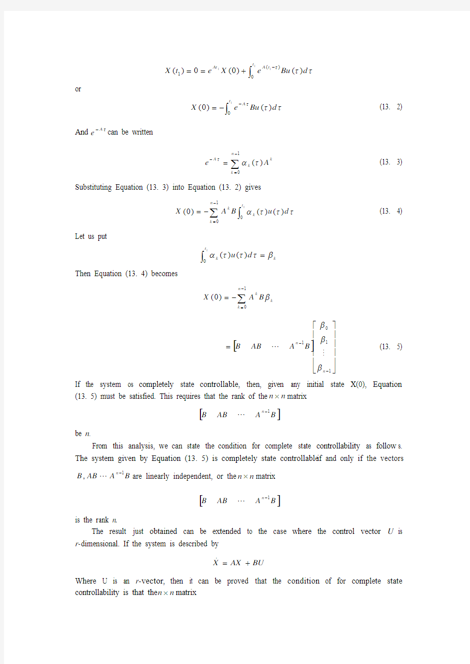
(13. 5) If the system os completely state controllable, then, given any initial state X(0), Equation
(13. 5) must be satisfied. This requires that the rank of the n n ?matrix
[]
B A
AB B
n 1
-
be n .
From this analysis, we can state the condition for complete state controllability as follow s. The system given by Equation (13. 5) is completely state controllable if and only if the vectors
B A
AB B n 1
,- are linearly independent, or the n n ?matrix
[]
B A
AB B
n 1
-
is the rank n.
The result just obtained can be extended to the case where the control vector U is r-dimensional. If the system is described by
BU AX X
+= Where U is an r -vector, then it can be proved that the condition of for complete state
controllability is that the n n ?matrix
[]
B A
AB B n 1
-
be of rank n , or contain n linearly independent column vectors. The matrix
[]
B A
AB
B
n 1
-
is commonly called the controllability matrix.
Complete Observability of Continuous-Time System
In this section we discuss the observability of linear systems. Consider the unforced system described by the following equations
AX X
= (13. 6) CX Y = (13. 7)
where X=state vector (n -vector)
Y=output vector (m -vector) A=n n ?matrix C=n m ?matrix
The system is said to be completely observable if every state )(0t X can be determined from the observation of Y(t) over a finite time interval,10t t t ≤≤. The system is, therefore, completely observable if every transition of the state eventually affects every element of the output vector. The concept of observability os useful in solving the problem or reconstructing unmeasurable state variable from measurable variables in the minimum possible length of time. In this section we treat only linear, time-invariant systems. Therefore, without loss of generality, we can assume that 00=t .
The concept of observability is very important because, in practice, the difficulty encountered with state feedback control is that some of the state variables are not accessible for direct measurement, with the result that it becomes necessary to estimate the unmeasurable state variables in order to construct the control signals.● Such estimates of state variables are possible of and only if the system is completely observable.
In discussion observability conditions, we consider the unforced system as given by Equation (13. 6) and (13. 7). The reasons for this are as follows, If the system is described by
Bu AX X
+= Bu CX Y +=
then
?
-+
=t
t A At
d Bu e
X e t X 0
)
()()0()(τττ
And Y(t) is
?++=-t
t A At
Du d Bu e
C X Ce
t Y 0
)
()()0()(τττ
Since the matrices A, B, C, and D are known and u(t) is also known,the last terms on
the right-hand side of this last equation are known quantities. Therefore, they may be subtracted from the observed value of Y(t). Hence, for investigating a necessary and sufficient condition for complete observability, it suffices to consider the system described by Equations (13. 6) and (13. 7).
Consider the system described by Equations (13. 6) and (13. 7). The output vector Y(t) is
)0()(X Ce
t Y At
=
And At e can be written as
∑-==
1
)(n k k
k
At
A t e α
Hence, we obtain
∑-==
1
)0()()(n t k
k
X CA t t Y α
or
)0()()0()()0()()(1
110X CA
t CAX t CX t t Y n n --+++=ααα (13. 8)
If the system is completely observable, then, given the output Y(t) over a time interval ≤≤t t 0 1t , X(0)is uniquely determined from Equation (13. 8). It can be shown that this requires the
rank of the n nm ?matrix
?????
???????-1n CA CA C to be n.
From this analysis we can state the condition for complete observability as follows.
The system described by Equation (13. 6) and (13. 7) is completely observable of and only is the n nm ?matrix
?????
???????-1n CA CA C is of rank n or has n linearly independent column vectors. This matrix is called the observability matrix.
Key Words and Terms
1. controllability n. 可控性
2. observability n. 可观测性
3. controllable adj. 可控的
4. observable adj. 可观测的
5. mathematical model 数学模型
6. property n. 性质,属性
7. continuous-time system 连续时间系统 8. generality n. 一般性,普遍性 9. rank n. 秩
10. linearly independent 线性无关 11. time-invariant system 时变系统 12. suffice v. 满足
Notes
Although most physic al systems are controllable an d observable, corresponding mathematical models may not possess the property of controllability and observability.
尽管大多数的物理系统都是可控的和可观测的,它们所对应的数学模型并不一定具有可控性和可观测性。
The system os said to be completely observable if every state )(0t X can be determined from the observation of Y(t) over a finite time interval,10t t t ≤≤.
如果在有限的时刻t ,10t t t ≤≤,从系统的输出Y(t)的观测中能确定每一个状态向量的初值)(0t x ,则称系统是完全可观测的。
● The concept of observability is very important because, in practice, the difficulty encountered with state feedback control is that some of the state variables are not accessible for direct measurement, with the result that it becomes necessary to estimate the unmeasurable state variables in order to construct the control signals.
可观测性的概念非常重要,在实际中,状态反馈控制中所遇到的困难在于,一些状态变量是不能够直接测量的,因此有必要估计不可测量的状态变量来构成控制信号。
encountered with state feedback control 为过去分词作定语,修饰the difficulty
that some of the state variables are not accessible for direct measurement 为表语从句。 that it becomes necessary to estimate the unmeasurable state variables in order to construct the control signal.为同位语从句,解释the result 。
Exercises
1. Consider the system defined by
u x x x x x
x
????
?
?????+????????????????????-----=??????????10210
1
110221321321
[]????
??????=32101
1x x x y Is the system completely state controllable? 2. Consider the system
????
?
???????????????=??????????32132113
120002x x x x x
x
The output is given by
[]???
?
??????=321111x x x y
Show that the system is not completely observable. 3. Please translate the following paragraph into Chinese.
A system is said to be controllable at time 0t if it is possible by means of an unconstrained control vector to transfer the system from any initial state )(0t X to any other state in a finite interval of time. A system is said to be observable at time 0t if,with the system in state )(0t X , it is possible to determine this state from observation of the output over a finite time
interval.
Unit 14 Internal Model Control
In the last chapter we presented several methods for tuning PID controllers and developed a model-based procedure (direct synthesis) to synthesize a controller that yields a desired closed-loop response trajectory. In this chapter, we first develop an "open-loop control" design procedure that then leads to the development of an internal model control (IMC) structure. There are a number of advantages to the IMC structure (and controller design procedure), compared with the classical feedback control structure. One is that it becomes very clear how process characteristics such as time delays and RHP zeros affect the inherent controllability of the process. IMCs are much easier to tune than are controllers in a standard feedback control structure.
After studying this chapter, the reader should be able to:
● Design internal model controllers for stable process (either minimum or non-minimum phase ●);
● Sketch the closed-loop response of the model is perfect; ● Derive the closed-loop transfer functions for IMC; ● Design IMC improved disturbances for IMC.
Introduction to Model-Based Control
In the previous chapters we focused on techniques to tune PID controllers. The closed-loop oscillation technique developed by Ziegler and Nichols did not require a mode of the process. Direct synthesis, however, was based the use of a process model and a desired closed-loop response to synthesize a control law; often this resulted in a controller with a PID structure.? In this chapter we develop a model-based procedure, where a process model is "embedded" in the controller. By explic itly using process know ledge, by virtue of the process model, improved performances can be obtained.
Consider the stirred-tank heater control problem shown in Figure 14. 1. We can use a model of the process to decide the heat flow (Q) that needs to be added to the process to obtain a desired temperature (T) trajectory, specified by the set-point (sp T ). A simple steady-state energy balance provides the steady-state heat flow needed to obtain a new steady-state temperature, for example.? By using a dynamic model, we can find the time-dependent heat profile needed to yield a particular time-dependent temperature profile.?
Assume that the chemical process is represented by a linear transfer function model, and that it is open-loop stable. The input-output relationship is shown in Figure 14. 2(a), where U(s) is the input variable (heat flow) and Y(s) is the output variable (temperature).
When the process is at steady state, and there are no disturbances, then the inputs and outputs are zero (since we are using deviation variables). Consider a desired change in the output Y(s); we refer to the desired value of Y(s) as the set-point, which is represented R(s). We wish to design an open-loop controller, Q(s), so that the relationship between R(s) and Y(s) has desirable dynamic characteristic (fast response without much overshoot, no off-set, etc.).The open-loop control system is shown in Figure 14. 2(b) (we may also wish to think of this as a feed-forward controller, based on set-point). We use Q(s) to represent the open-loop controller transfer function, to emphasize that it is a different type of controller than the feedback controller of previous chapters.
Using block diagram analysis, we find the following relationship between the set-point and the output
)()()()(s R s Q s G s Y p = (14. 1)
Static Control Law
The simplest controller will result if Q(s) is constant. Let p k represent this constant. As
an example, consider a first-order process,)(1
)(s R s k s G p p
p +=τ. Then the relationship
between R(s) and Y(s) is
)(1
)(s R s k k s Y p p
q +=
τ
To obtain a desirable response,p
q k k 1=
;offset will result otherwise. We can see this from the
final-value theorem. Consider a step set-point change, of magnitude 1R
s
R s k k s Y p p
q 1
1)(+=
τ (14. 2)
From the final-value theorem
10
)(lim )(lim R k k s sY t y q p s t ==→∞
→
And for no offset, we require that p
q k k 1=. We can also find the time-domain solution to
Equation (14. 2)
)1()(/1p
t q p e
R k k t y τ
--=
Again, we can see that p
q k k 1=
is necessary for offset-free performance. Notice also that
the speed of response is the same as the time constant of open-loop process. In order to "speed- up" the response, we must use dynamic control law, as developed in the next section.
Dynamic Control Law
Better control can be obtained of the controller, Q(s), is dynamic rather than static. Indeed, we find that if
)
(1)(s G s Q p =
(14. 3)
then the relationship between R(s) and Y(s) is
)()()
(1)
()()()()(s R s R s G s G s R s Q s G s Y p p p ===
That is, we have perfect control, since the output perfectly tracks the set-point! For a first- order process, the controller is
p
p p k s s G s Q 1)
(1)(+=
=
τ
Although this is mathematically possible, perfect control is unachievable in practical application. Consider the signals in and out of the control block, shown in Figure 2(b). Since the transfer function relationship between R(s) and U(s) is, for this example,
)(1)()()(s R k s s R s Q s U p
p +=
=τ (14. 4)
The differential equation that corresponds to Equation (14. 4) is
)(1)(t r k dt
dr k t u p
p p +
=
τ
From a practical point of view, it is impossible to take an exact derivative of r(t), particularly if a discontinuous step set-point change is made.
Here we use the inverse Laplace transfer to solve Equation (14. 4) for u(t), when there is a step change in r(t)
s
k R k R s U p p
p 1)(11+
=
τ
A table of Laplace transform can be used to find the time-domain solution
p
p
p k R t k R t u 11)()(+
=
δτ
where )(t δis the impulse function, which has infinite height, infinitesimal width, and unit area. Since this is hard to understand conceptually, you probably realize that it is impossible to implement exactly. Think about how you would approximate it.
Key Words and Terms
1. internal model control 内模控制
2. embed adj. 嵌入的
3. by virtue of 依靠......的力量,借助,凭借
4. flow n. 流量
5. overshoot n. 超调量
6. off-set n. 误差、偏差
7. feed-forward n. 前馈
8. final-value theorem 终值定理
Notes
本文选自Prentic e Hall 出版社出版的Process Control (Modeling, Design, and Simulation),作者B. Wayne Bequette 。
One is that it becomes very clear how process characteristics such as time delays and RHP zeros affect the inherent controllability of the process.
其中一个优点是,诸如时滞、右半平面零点等过程特性如何影响过程的内在可控性的问题会清楚地显现出来。
RHP zero 右半平面(Right of Half Plane )零点。 ● non-minimum phase 非最小相位(系统),指在复平面右半平面有零极点的系统。 ? Direct synthesis, however, was based the use of a process model and a desired closed- loop response to synthesize a control law; often this resulted in a controller with a PID structure.
然而,直接综合法是使用过程模型和期望的闭环响应来综合控制器,经常可以得到具有PID 结构的控制器。
? A simple steady-state energy balance provides the steady-state heat flow needed to obtain a new steady-state temperature, for example.
例如。一个简单的稳态能量平衡关系可以给出为达到新的稳态温度所需要的稳态热流量。
? By using a dynamic model, we can find the time-dependent heat profile needed to yield a particular time-dependent temperature profile.
为了产生一个特定的温度—时间曲线,我们可以通过使用动态模型而得到必须的热流量—时间曲线。
Exercises
1. Please translate the last three paragraphs in Chinese (From "From a practice of view. . ." to ". . . would approximate it").
2. Does the static control law produces any steady state error if p
q k k 1
?
3. When was the PID controller invented?(The fact does not exist in this text.)
4. Please consider that why the order of translation of notation ? is different from the original English.
实验十 系统能控性与能观性分析
实验十 系统能控性与能观性分析 一、实验目的 1. 通过本实验加深对系统状态的能控性和能观性的理解; 2. 验证实验结果所得系统能控能观的条件与由它们的判据求得的结果完全一致。 二、实验设备 同实验一。 三、实验内容 1. 线性系统能控性实验; 2. 线性系统能观性实验。 四、实验原理 系统的能控性是指输入信号u 对各状态变量x 的控制能力。如果对于系统任意的初始状态,可以找到一个容许的输入量,在有限的时间内把系统所有的状态变量转移到状态空间的坐标原点。则称系统是能控的。 系统的能观性是指由系统的输出量确定系统所有初始状态的能力。如果在有限的时间内,根据系统的输出能唯一地确定系统的初始状态,则称系统能观。 对于图10-1所示的电路系统,设i L 和u c 分别为系统的两个状态变量,如果电桥中 4 32 1R R R R ≠,则输入电压u 能控制i L 和u c 状态变量的变化,此时,状态是能控的;状态变量 i L 与u c 有耦合关系,输出u c 中含有i L 的信息,因此对u c 的检测能确定i L 。即系统能观的。 反之,当 4 32 1R R = R R 时,电桥中的c 点和d 点的电位始终相等, u c 不受输入u 的控制, u 只能改变i L 的大小,故系统不能控;由于输出u c 和状态变量i L 没有耦合关系,故u c 的检测不能确定i L ,即系统不能观。 1.1 当 4 32 1R R R R ≠时 u L u i R R R R C R R R R R R R R L R R R R R R C R R R R R R R R L u i C L C L ? ??? ? ??+? ??? ???????? ??+++-+- +- ? ?+- +- +++- =???? ??01)11(1)( 1 ) ( 1)( 14321434 3212 14 342 124 3432 121 (10-1) y=u c =[0 1] ??? ? ? ??c L u i (10-2) 由上式可简写为 bu Ax x += cx y = 式中???? ??=C L u i x ???? ?? ? +++- +-+- ? ?+-+-++ +-=)11( 1)( 1 )( 1)( 1 432 1434 3212 14 342 124 343212 1R R R R C R R R R R R R R L R R R R R R C R R R R R R R R L A
系统的能控性、能观测性、稳定性分析
实 验 报 告 课程 线性系统理论基础 实验日期 年 月 日 专业班级 学号 同组人 实验名称 系统的能控性、能观测性、稳定性分析及实现 评分 批阅教师签字 一、实验目的 加深理解能观测性、能控性、稳定性、最小实现等观念。掌 握如何使用MATLAB 进行以下分析和实现。 1、系统的能观测性、能控性分析; 2、系统的稳定性分析; 3、系统的最小实现。 二、实验内容 (1)能控性、能观测性及系统实现 (a )了解以下命令的功能;自选对象模型,进行运算,并写出结 果。 gram, ctrb, obsv, lyap, ctrbf, obsvf, minreal ; (b )已知连续系统的传递函数模型,18 2710)(23++++=s s s a s s G ,当a 分别取-1,0,1时,判别系统的能控性与能观测性;
(c )已知系统矩阵为???? ??????--=2101013333.06667.10666.6A ,??????????=110B ,[]201=C ,判别系统的能控性与能观测性; (d )求系统18 27101)(23++++= s s s s s G 的最小实现。 (2)稳定性 (a )代数法稳定性判据 已知单位反馈系统的开环传递函数为:) 20)(1()2(100)(+++=s s s s s G ,试对系统闭环判别其稳定性 (b )根轨迹法判断系统稳定性 已知一个单位负反馈系统开环传递函数为 ) 22)(6)(5()3()(2+++++=s s s s s s k s G ,试在系统的闭环根轨迹图上选择一点,求出该点的增益及其系统的闭环极点位置,并判断在该点系统闭环的稳定性。 (c )Bode 图法判断系统稳定性 已知两个单位负反馈系统的开环传递函数分别为 s s s s G s s s s G 457.2)(,457.2)(232231-+=++= 用Bode 图法判断系统闭环的稳定性。 (d )判断下列系统是否状态渐近稳定、是否BIBO 稳定。 []x y u x x 0525,100050250100010-=????? ?????+??????????-=
系统的能控性与能观性分析及状态反馈极点配置
实 验 报 告 课程 自动控制原理 实验日期 12 月26 日 专业班级 姓名 学号 实验名称 系统的能控性与能观性分析及状态反馈极点配置 评分 批阅教师签字 一、实验目的 加深理解能观测性、能控性、稳定性、最小实现等观念,掌握状态反馈极点配置方法,掌握如何使用MATLAB 进行以下分析和实现。 1、系统的能观测性、能控性分析; 2、系统的最小实现; 3、进行状态反馈系统的极点配置; 4、研究不同配置对系统动态特性的影响。 二、实验内容 1.能控性、能观测性及系统实现 (a )了解以下命令的功能;自选对象模型,进行运算,并写出结果。 gram, ctrb, obsv, lyap, ctrbf, obsvf, mineral ; (b )已知连续系统的传递函数模型,18 2710)(23++++= s s s a s s G , 当a 分别取-1,0,1时,判别系统的能控性与能观测性;
(c )已知系统矩阵为??????????--=2101013333.06667.10666.6A ,?? ??? ?????=110B ,[]201=C ,判别系统的能控性与能观测性; (d )求系统18 27101 )(2 3++++=s s s s s G 的最小实现。 2.实验内容 原系统如图1-2所示。图中,X 1和X 2是可以测量的状态变量。 图1-2 系统结构图 试设计状态反馈矩阵
,使系统加入状态反馈后其动态性能指标满足给定的要求: (1) 已知:K=10,T=1秒,要求加入状态反馈后系统的动态性能指标为: σ%≤20%,ts≤1秒。 (2) 已知:K=1,T=0.05秒,要求加入状态反馈后系统的动态性能指标为: σ%≤5%,ts≤0.5秒。 状态反馈后的系统,如图1-3所示:
能控性和能观性
第五章能控性和能观性 5-1 离散时间系统的可控性 定义设单输入n阶线性定常离散系统状态方程为: ……………………………………………………………(5-1) 其中 X(k)__n维状态向量; u(k) __1维输入向量; G__n×n系统矩阵; h__n×1输入矩阵; 如果存在有限步的控制信号序列u(k),u(k+1),…,u(N-1),使得系统第k步上的状态X(k) 能在第N步到达零状态,即X(N)=0,其中N是大于k的有限正整数,那么就说系统第k步上的状态X(k)是能控的;如果第k步上的所有状态都能控,则称系统(5-1)在第k步上是完全能控的。进一步,如果系统的每一步都是可控的,那么称系统(5-1)完全可控,或称系统为能控系统。 定理1单输入n阶离散系统(5-1)能控的充要条件是,能控判别阵: 的秩等于n,即:
……………………………………(5-2) 【证】:因为系统为一线性系统,不妨设系统从任一初态X(0)开始,在第n步转移到零状态,即X(n)=0。根据离散状态方程的解: ……………………………………………………(5-3) 因为X(n)=0,所以: 写成矢量形式: …………………………………(5-4) 从线性代数知识可知,上式中对于任意的初始状态X(0),要求都存在一组控制序列u(0),u(1),…,u(n-1)的充要条件是阶系数矩阵 满秩,即
【例5-1】设离散系统状态方程为: 判断系统的可控性。 解: M是一方阵,其行列式为: 所以系统能控判别阵满秩,系统可控。 定理2考虑多输入离散系统情况,假如线性定常离散系统状态方程为: ………………………………………………………(5-5) 其中X为阶矢量,U为阶矢量,G为阶矩阵,H为n×r阶能控矩阵。那么离散系统(5-5)能控的充要条件是:能控判别阵 的秩等于n。 (证略)。
(整理)控制系统的能控性和能观测性
第三章 控制系统的能控性和能观测性 3-1能控性及其判据 一:能控性概念 定义:线性定常系统(A,B,C),对任意给定的一个初始状态x(t 0),如果在t 1> t 0的有限时间区间[t 0,t 1]内,存在一个无约束的控制矢量u(t),使x(t 1)=0,则称系统是状态完全能控的,简称系统是能控的。 可见系统的能控性反映了控制矢量u(t)对系统状态的控制性质,与系统的内部结构和参数有关。 二:线性定常系统能控性判据 设系统动态方程为: x 2不能控 y 2则系统不能控 ,若2121,C C R R ==?? ?+=+=Du Cx y Bu Ax x
设初始时刻为t 0=0,对于任意的初始状态x(t 0),有: 根据系统能控性定义,令x(t f )=0,得: 即: 由凯莱-哈密尔顿定理: 令 上式变为: 对于任意x(0),上式有解的充分必要条件是Q C 满秩。 判据1:线性定常系统状态完全能控的充分必要条件是: ?-+=f t f f f d Bu t x t t x 0)()()0()()(τττφφ??---=--=-f f t f f t f f d Bu t t d Bu t t x 0 1)()()()()()()0(τ ττφφτττφφ?--=f t d Bu x 0)()()0(τττφ∑-=-==-1 )()(n k k k A A e τατφτ ∑??∑-=-=-=-=1 01 )()()()()0(n k t k k t n k k k f f d u B A d Bu A x τ τταττταk t k u d u f =? )()(ττταU Q u u u u B A B A AB B Bu A x c k n n k k k -=???? ? ?? ?????????-=-=--=∑ 321121 ],,,[)0(
实验三 利用Matlab分析能控性和能观性
实验三利用Matlab分析能控性和能观性 实验目的:熟练掌握利用Matlab中相关函数分析系统能控能观性、求取两种标准型、系统的结构分解的方法。 实验内容: 1、能控性与能观性分析中常用的有关Matlab函数有: Size(a,b) 获取矩阵的行和列的数目 Ctrb(a,b) 求取系统能控性判别矩阵 Obsv(a,c) 求取能观性判别矩阵 Rank(t) 求取矩阵的秩 Inv(t) 求矩阵的逆 [abar,bbar,cbar,t,k]=ctrbf(a,b,c) 对系统按能控性分解,t为变换阵,k为各子系统的秩[abar,bbar,cbar,t,k]=obsvf(a,b,c) 对系统按能观性分解 2、利用Matlab判定系统能控性和能观性 A、求取判别矩阵的秩,而判别矩阵可用两种方法得到: M=ctrb(a,b) 或者M=[b,a*b,a^2*b,……] B、将系统变换为对角线型或者约当标准型,根据结果直接判断。化为标准型可以使用第 一次实验中介绍的ss2ss、canon等函数。 3、化为能控标准型和能观标准型 如:>> a=[1 0 1;0 1 0;1 0 0]; >> b=[0 1 1]'; >> c=[1 1 0]; >> m=ctrb(a,b) m = 0 1 1 1 1 1 1 0 1 >> n=length(a);tc1=eye(n);tc2=eye(n); >> tc1(:,1)=m(:,3) tc1 = 1 0 0 1 1 0 1 0 1 >> tc1(:,2)=m(:,2) tc1 = 1 1 0 1 1 0 1 0 1
>> tc1(:,3)=m(:,1) tc1 = 1 1 0 1 1 1 1 0 1 >> qc=rank(m) qc = 3 >> den=poly(a) den = 1.0000 - 2.0000 0.0000 1.0000 >> tc2(2,1)=den(2) tc2 = 1 0 0 -2 1 0 0 0 1 >> tc2(3,2)=den(2);tc2(3,1)=den(3) tc2 = 1.0000 0 0 -2.0000 1.0000 0 0.0000 -2.0000 1.0000 >> tc3=tc1*tc2;tc4=inv(tc3); >> a1=tc4*a*tc3 a1 = -0.0000 1.0000 0.0000 0.0000 0 1.0000 -1.0000 0.0000 2.0000 >> b1=tc4*b b1 = 0.0000 1.0000 >> c1=c*tc3 c1 = -2.0000 0 1.0000 参照该例,掌握其他标准型的求解办法。 4、系统的结构分解 A 、 找到变换矩阵c R 或者o R ,利用线性变换进行结构分解。
能控性及能观测性
第三章:控制系统的能控性及能观测性(第五讲) 内容介绍: 能控性和能观测性定义、判据、对偶关系、标准型、结构分解。 能控性和能观测性是现代控制理论中最基本概念, 是回答:“输入能否控制状态的变化”及 “状态的变化能否由输出反映出来”这样两个问题。 换句话说,能控性是“能否找到一向量u(t)有效控制x(t)变化”。 能观测性问题是:“能否通过输出y(t)观测到状态的变化。” 一、能控性定义及判据 给出一个多变量系统(多输入、多输出) 若系统G(s)在适当的控制u(t)作用下,每个状态都受影响,亦在有限的时间内能使系 统G 由任意初始状态转移到零状态,或者说在有限的时间内能使系统由零状态转移到任意指定状态。 这说明: 输入对状态的控制能力强,反之若 G 的某一状态根本不受影响,那么在有限时间内就 无法利用控制使这个状态变量发生变化。说明输入对状态控制能力差。 可见:反映输入对状态控制能力的概念是能控性概念。 1. 定义:若对系统,在时刻的任意状态x()都存在一个有限的时间区间( ξ t t ,0)(0 t t ?ξ) 和定义在 []ξ t ,t 0上适当的控制u(t),使在u(t)作用下x()=0。 则称系统在时刻是状态能控的。 如果系统在有定义的时间区域上的每一时刻都能控,称系统为完全能控。 ()x u x 01011012=??? ? ??+???? ??-=考查能控性? 状态变量图(信号流图): y 2 由于u 的作用只影响不影响,故()t x 2为不能控。 某一状态不能控,则称系统不能控。 2.判据: u 1 : y 1 :
对线性定常系统=Ax+Bu , 若对某一时刻能控,则称系统完全能控。 设: p 输出 n n A *、p n B *、n m C * 给出一定理: 由=Ax+Bu 所描述的系统是状态完全能控的必要且充分条件为 下列n ×np 阵的秩等于n 。 =B AB ……B A n 1 -称为能控性阵。 换言之:系统的状态完全能控的必要且充分的条件是能控性阵的秩为n 。 定理证明可参考书。 状态完全能控称“(A ,B )能控” 例: u x x ???? ??-+???? ??--=42314310 224310 ?? ??? ??--=A 则系统为二阶 ,n=2 B AB ……B A n 1 -=????? ?-AB )B (4231=??? ???---7114342 3 1 rankB AB]=2=n 4 231 ≠-有二阶子式 秩的确定:最高阶不为0子式的阶次 可知:系统的状态能控,称(A ,B )能控 信号流图: 顺便: 计算的行数小于列数的矩阵的秩时,应用下列关系较方便: rank()=rank(T c c Q Q )T c c Q Q 为方阵其秩计算较简单。 利用判定能控性方法被广泛采用。 新出现的PBH 秩检验法也可用于能控性判别。 =Ax+Bu y=cx
线性控制系统的能控性和能观性
第三章 线性控制系统的能控性和能观性 注明:*为选做题 3-1 判别下列系统的能控性与能观性。系统中a,b,c,d 的取值对能控性与能观性是否有关,若有关其取值条件如何? (1)系统如图所示。 题3-1(1)图 系统模拟结构图 (2)系统如图所示。 题3-1(2)图 系统模拟结构图 (3)系统如下式: 1122331122311021010000200000x x x a u x x b x x y c d x y x ?????-?????? ? ??? ? ?=-+ ??? ? ? ??? ? ?-?????? ??? ?????? ?= ? ? ????? ??? 3-2* 时不变系统:
311113111111x x u y x ? -????=+ ? ?-??????= ?-?? 试用两种方法判别其能控性与能观性。 3-3 确定使下列系统为状态完全能控和状态完全能观的待定常数,i i αβ。 (1)0∑()1201,,1101A b C αα????===- ? ????? (2) ()230021103,,001014A b C ββ???? ? ?=-== ? ? ? ?-???? 3-4* 线形系统的传递函数为: ()()32102718 y s s a u s s s s +=+++ (1)试确定a 的取值,使系统为不能控或不能观的。 (2)在上述a 的取值下,求使系统为能控状态空间表达式。 (3)在上述a 的取值下,求使系统为能观的状态空间表达式。 3-5* 试证明对于单输入的离散时间定常系统(,)T G h =∑,只要它是完全能控 的,那么对于任意给定的非零初始状态0x ,都可以在不超过n 个采样周期的时间内,转移到状态空间的原点。 3-6 已知系统的微分方程为: 61166y y y y u ?????? +++= 试写出其对偶系统的状态空间表达式及其传递函数。 3-7 已知能控系统的状态方程A,b 阵为: 121,341A b -????== ? ????? 试将该状态方程变换为能控标准型。 3-8已知能观系统的状态方程A,b ,C 阵为: ()112,,11111A b C -????===- ? ????? 试将该状态空间表达式变换为能观标准型。 3-9 已知系统的传递函数为: 2268()43 s s W s s s ++=++
现代控制理论基础_周军_第三章能控性和能观测性
3.1 线性定常系统的能控性 线性系统的能控性和能观测性概念是卡尔曼在1960年首先提出来的。当系统用状态空间描述以后,能控性、能观测性成为线性系统的一个重要结构特性。这是由于系统需用状态方程和输出方程两个方程来描述输入-输出关系,状态作为被控量,输出量仅是状态的线性组合,于是有“能否找到使任意初态转移到任意终态的控制量”的问题,即能控性问题。并非所有状态都受输入量的控制,有时只存在使任意初态转移到确定终态而不是任意终态的控制。还有“能否由测量到的由状态分量线性组合起来的输出量来确定出各状态分量”的问题,即能观测性问题。并非所有状态分量都可由其线性组合起来的输出测量值来确定。能控性、能观测性在现代控制系统的分析综合中占有很重要的地位,也是许多最优控制、最优估计问题的解的存在条件,本章主要介绍能控性、能观测性与状态 空间结构的关系。 第一节线性定常系统的能控性 能控性分为状态能控性、输出能控性(如不特别指明便泛指状态能控性)。状态能控性问题只与状态方程有关,下面对定常离散系统、定常连续系统分别进行研究(各自又包含单输入与多输入两种情况): 一、离散系统的状态可控性 引例设单输入离散状态方程为: 初始状态为: 用递推法可解得状态序列:
可看出状态变量只能在+1或-1之间周期变化,不受的控制,不能从 初态转移到任意给定的状态,以致影响状态向量也不能在作用下转移成任意给定的状态向量。系统中只要有一个状态变量不受控制, 便称作状态不完全可控,简称不可控。可控性与系统矩阵及输入矩阵密切相关,是系统的一种固有特性。下面来进行一般分析。 设单输入离散系统状态方程为: (3-1) 式中,为维状态向量;为纯量,且在区间是常数,其 幅值不受约束;为维非奇异矩阵,为系统矩阵;为维输入矩 阵:表示离散瞬时,为采样周期。 初始状态任意给定,设为;终端状态任意给定,设为,为研究方 便,且不失一般性地假定。 单输入离散系统状态可控性定义如 下:
指导书系统能控性与能观性分析
实验六 系统能控性与能观性分析 一、实验目的 1. 通过本实验加深对系统状态的能控性和能观性的理解; 2. 验证实验结果所得系统能控能观的条件与由它们的判据求得的结果完全一致。 二、实验设备 同实验一。 三、实验内容 1. 线性系统能控性实验; 2. 线性系统能观性实验。 四、实验原理 系统的能控性是指输入信号u 对各状态变量x 的控制能力。如果对于系统任意的初始状态,可以找到一个容许的输入量,在有限的时间内把系统所有的状态变量转移到状态空间的坐标原点。则称系统是能控的。 系统的能观性是指由系统的输出量确定系统所有初始状态的能力。如果在有限的时间内,根据系统的输出能唯一地确定系统的初始状态,则称系统能观。 对于图6-1所示的电路系统,设i L 和u c 分别为系统的两个状态变量,如果电桥中 4 3 21R R R R ≠,则输入电压u 能控制i L 和u c 状态变量的变化,此时,状态是能控的;状态变量i L 与u c 有耦合关系,输出u c 中含有i L 的信息,因此对u c 的检测能确定i L 。即系统能观的。 反之,当 4 3 21R R =R R 时,电桥中的c 点和d 点的电位始终相等, u c 不受输入u 的控制,u 只能改变i L 的大小,故系统不能控;由于输出u c 和状态变量i L 没有耦合关系,故u c 的检测不能确定i L ,即系统不能观。 1.1 当4 321R R R R ≠时 u L u i R R R R C R R R R R R R R L R R R R R R C R R R R R R R R L u i C L C L ??? ? ? ??+???? ??????????+++-+-+- ??+-+-+++-=???? ??01)11(1)(1) (1)( 143214343212 14342124343212 1 (6-1) y=u c =[0 1] ??? ? ? ??c L u i (6-2) 由上式可简写为 bu Ax x += cx y = 式中???? ??=C L u i x ???? ? ?? +++-+- +- ? ?+-+-+++-=)11(1)( 1)(1)(14321434 32121434212 4343212 1R R R R C R R R R R R R R L R R R R R R C R R R R R R R R L A
系统的能控性与能观性分析及状态反馈极点配置要点
信控学院上机实验 实验报告 课程自动控制原理实验日期12 月26 日 专业班级姓名学号 实验名称系统的能控性与能观性分析及状态反馈极点配置评分 批阅教师签字 一、实验目的 加深理解能观测性、能控性、稳定性、最小实现等观念,掌握状态反馈极点配置方法,掌握如何使用MATLAB进行以下分析和实现。 系统的能观测性、能控性分析;、12、系统的最小实现; 3、进行状态反馈系统的极点配置; 4、研究不同配置对系统动态特性的影响。 二、实验内容 1.能控性、能观测性及系统实现 (a)了解以下命令的功能;自选对象模型,进行运算,并写出结果。 gram, ctrb, obsv, lyap, ctrbf, obsvf, mineral; s?a?)G(s,)已知连续系统的传递函数模型,b(32?27s?18ss?10当a 分别取-1,0,1时,判别系统的能控性与能观测性; 页共页第 信控学院上机实验 6.666?10.6667?0.33330?????????11A1?B0已知系统矩阵为(,,c)????????0121??????,判别系统的能控性与能观测性;21?C0s?1?s)G(的最小实现。)求系统(d 32?27s10s?s18? 2.实验内容是可以测量的状态变量。和原系统如图1-2所示。图中,XX21 图1-2 系统结构图 试设计状态反馈矩阵使系统加入状态反馈后其,: 动态性能指标满足给定的要求 (1) 已知:K=10,T=1秒,要求加入状态反馈后系统的动态性能指标为:
σ%≤20%,ts≤1秒。 (2) 已知:K=1,T=0.05秒,要求加入状态反馈后系统的动态性能指标为: σ%≤5%,ts≤0.5秒。 状态反馈后的系统,如图1-3所示: 页共页第 信控学院上机实验 状态反馈后系统结构图1-3 图并检验系统分别观测状态反馈前后两个系统的阶跃响应曲线,的动态性能指标是否满足设计要求。 三、实验环境台;1、计算机1套。MATLAB6.5软件12、 四、实验原理(或程序框图)及步骤、系统能控性、能观性分析1 设系统的状态空间表达式如下:?xBuAx???pnm Ryx?R?uR??DuCxy???(1-1)×为p×m维输入矩阵;C为×其中A为nn维状态矩阵;Bn 0。维传递矩阵,一般情况下为为n维输出矩阵;Dp×m(1-2)系统的传递函数阵和状态空间表达式之间的关系如式所示:页共页第 信控学院上机实验 num((s)?1D?sI?(s)?A)B?C(G)sden((1-2) num)(s中,式(1-2)表示传递函数阵的分子阵,其维数是p×)(sden降幂排列的 后,各表示传递函数阵的分母多项式,按s;m 项系数用向量表示。系统的能控性、能观测性分析是多变量系统设计的基础,包括能控性、能观测性的定义和判别。,1-1)系统状态能控性定义的核心是:对于线性连续定常系统()内,t-t 若存在一个分段连续的输入函数u(t),在有限的时间(01,则称此状态)x(tx(t)转移至预期的终端能把任一给定的初态10是能控的。若系统所有的状态都是能控的,则称该系统是状态完全能控的。种:一般判别和直接判别法,后2状态能控性判别方法分为是对角标准形或约当标准形的系统,状A者是针对系统的系数阵态能控性判别时不用计算,应用公式直接判断,是一种直接简易法;前者状态能控性分为一般判别是应用最广泛的一种判别法。状态能控性判别式为: ??1?n BRankB?RankQABAn??c)(1-3,1-1)系统状态能观测性的定义:对于线性连续定常系统(?的测量值,y(t)]上的t 第3章 能控性与能观性分析 教材【1】:《现代控制理论》,俞立编著. 清华大学出版社,2007年4月 主要参考书: 【2】《现代控制理论简明教程》,许世范等,中国矿业大学出版社,1996年1月第1版; 【3】《现代控制理论与工程》,东南大学 王积伟 主编 高等教育出版社,2003年2月第1版,研究生用书。 作业:9087P P -习题3.1;3.3;3.4;3.11;3.12;3.13;3.14;3.25 现代控制理论中,用状态空间方法描述系统,将系统的的输出-输入关系分成两部分: ① 系统的控制输入)(t u 对状态)(t x 的影响—由状态方程描述; ② 系统输出)(t y 与状态)(t x 的关系—由输出方程描述。 1960年,Kalman 根据“控制输入对状态的影响”首先提出了系统状态的能控性问题,根据“输出与状态的关系”提出了系统状态的能观性问题。 ① 能控性:输入)(t u 能否通过“状态方程”引起系统任一状态)(t x i 的变化 )(t x i ?能控性描述通过输入)(t u 对系统状态)(t x 的控制能力; ② 能观性:系统任一状态)(t x i 的变化能否通过“输出方程”引起输出) (t y 的变化?或者由输出)(t y 的变化能否通过“输出方程”确定系统所有状 态变量)(t x i ,能观性描述通过输出)(t y 对系统状态)(t x 的测辨能力。 3.1 系统的能控性 3.1.1 能控性的定义和性质 系统能控性定义:在初始时刻0t t =时,对系统施加控制)(t u 使系统状态 )(t x 发生变化,并且输出)(t y ,)()()()()(t u t B t x t A t x += ,)()()(t x t C t y =,0t t ≥ 如果在有限时间T t t ≤≤0内存在容许(满足∞3.能控性与能观性分析
- 能控性和能观性分析
- 第四章 线性系统的能控性和能观性
- 现代控制理论能控性、能观测性
- 系统的能控性与能观性分析及状态反馈极点配置.
- 线性控制系统的能控性和能观性
- 第三章 控制系统的能控性与能观性PPT课件
- 线性系统的能控性和能观性
- 第3章 线性系统的能控性与能观测性1
- 控制系统的能控性和能观测性讲课资料
- 第3章 线性控制系统的能控性和能观性20151015 - 副本
- 第3章 控制系统的能控性和能观性
- 现代控制理论_线性控制系统的能控性与能观性基础知识47页PPT
- 控制系统的能控性与能观性
- 实验十 系统能控性与能观性分析
- 系统的能控性与能观性分析及状态反馈极点配置要点
- 41线性系统的能控性和能观性
- 系统的能控性与能观性分析及状态反馈极点配置
- 控制系统的能控性和能观性 (I)
- 第三章线性系统的能控性与能观性
- 第四章 能控性和能观测性